8. Beamline automation

Caution

Spreadsheets with version number earlier than 13 will not work as of 1 March, 2024.

BMM currently supports five categories of spreadsheet-based automation:

1. Sample wheels (spreadsheet)

2. Linkam stage temperature control (spreadsheet)

3. LakeShore 331 controller for Displex cryostat (spreadsheet)

4. Glancing angle stage (spreadsheet)

5. Generic XY and XYZ grids (spreadsheet)

The latest spreadsheets for each of these can always be found at NSLS-II-BMM/profile_collection

Each of the spreadsheets looks much like this, although there are some differences in the columns corresponding to the different instruments.

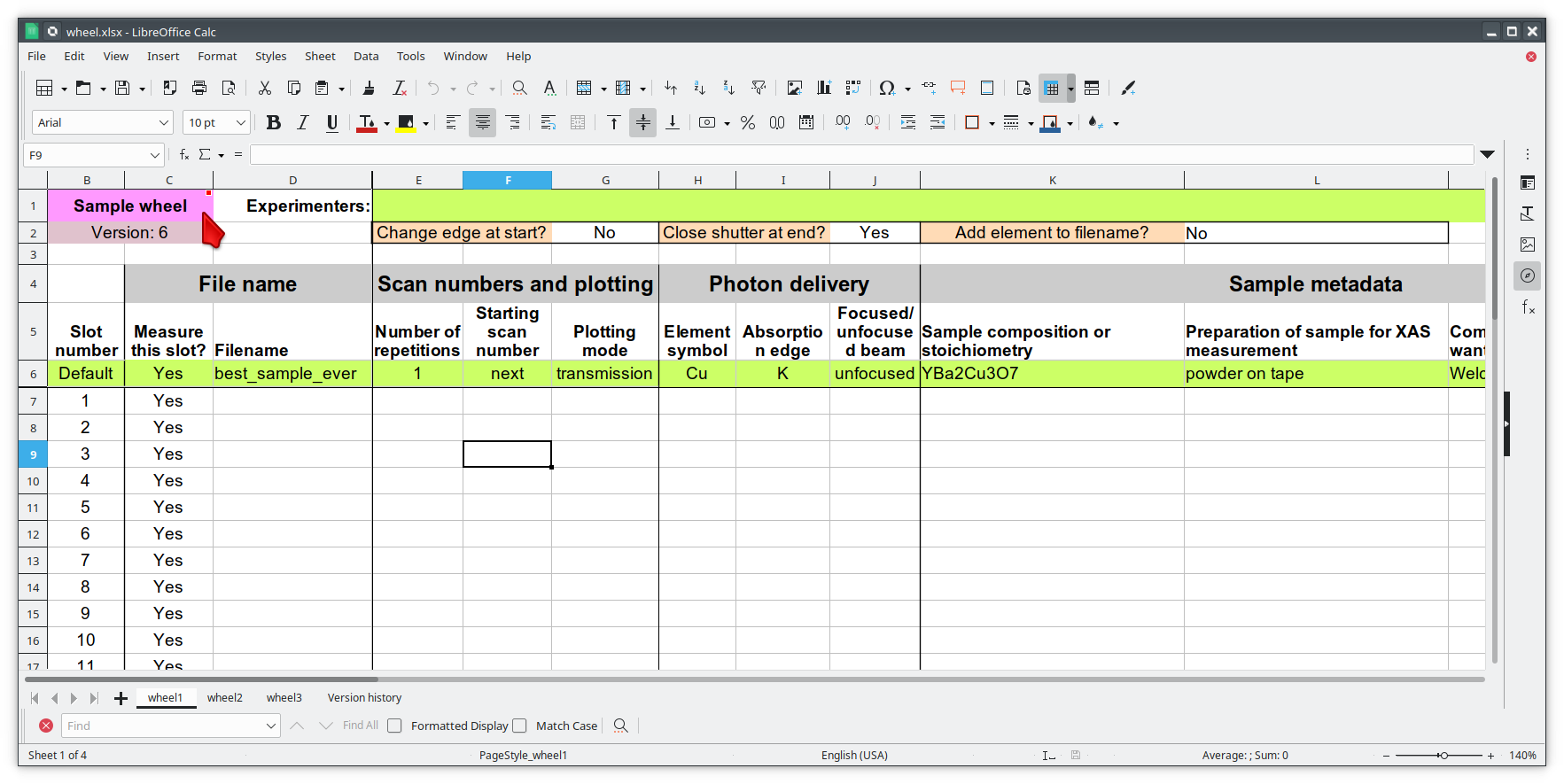
Fig. 8.1 Example spreadsheet for running an experiment from a wheel with a single sample ring.

Make sure you are using the most up-to-date version of the spreadsheet.

Note

The current spreadsheet version is 13, as of 29 February, 2024. You should always use a current spreadsheet.

Caution

Spreadsheets with version number earlier 13 will not work as of 1 March, 2024.

8.1. Common features

8.1.1. Default information

All the spreadsheets use the concept of “default” scan information, that is, information that is expected to be used for most or all of the indicated measurements. In Figure 8.1, the defults are entered into the row with the green background. All rows underneath the green line are used to describe individual measurements.

For an individual measurement, if a white cell is left blank, the default value from the corresponding green cell will be used. If a white cell is filled in, that value will be used for that measurement.

8.1.2. Experimenters

The other green part of the spreadsheet is a cell for entering the names of all the experimenters involved in the measurement.

This should always be filled in. Doing so allows for the possibility of searching BMM’s master database for data associated with a particular user.

8.1.3. Measurement options

Beneath the experimenter cell, there are three drop-down menus for setting aspects of the sequence of measurements described on the spreadsheet tab.

1. A yes/no menu for forcing Bluesky to run the change_edge() command at the beginning of the measurement sequence.

2. A yes/no menu for telling Bluesky to close the shutter at the end of the measurement sequence.

3. A menu of options for modifying filenames to contain information about things like absorber element, edge symbol, LInkam stage temperature, and so on. This simplifies data entry into the filename column of the spreadsheet.

4. A place for specifying the number of repetitions of the entire spreadsheet. This is different from the column labeled “repetitions”, which specifies the number of repeated XAS scans of the sample in that row of the spreadsheet.

8.1.4. Fine tuning sample position and slits

On the right hand side of each spreadsheet, there are columns for specifying specific positions for sample X and Y and for slit width and height. This allows you to fine tune the sample position and beam size on a per-sample basis.

The motor grid spreadsheet offers three columns for specifying motor positions. The motors associated with those columns are user-select-able. In this way, a grid over any beamline motor can programmed.

The glancing angle spreadsheet has the columns for specifying slit width and height. It also has columns for specifying sample Y and pitch (X and pitch when in perpendicular mode) when manual alignment rather than automated alignment is selected. There is no column for specifying the X position (or Y when in perpendicular mode) as use of the glancing angle stage presumes that all the samples are mounted at the centers of the spinners.

8.1.5. Selecting a spreadsheet

All spreadsheets are imported using the xlsx() command. The spreadsheets are self-identifying. Every spreadsheet has an identifying string spanning cells B1:C1. This is the cell with the pink background.

Caution

Never change the text in the pink cell or your spreadsheet will likely be interpreted incorrectly.

To convert a spreadsheet into a macro then run the macro, do the following:

xlsx()

This will show a numbered list of all .xlsx files in your data folder, something like this:

Select your xlsx file:

  1: 20210127-KB1.xlsx
  2: 20210127-KB3.xlsx
  3: 20210128-KB2.xlsx
  4: 20210128-KB4.xlsx
  5: 20210128-KB5.xlsx
  6: wheel_template.xlsx

  r: return

Select a file >

Select the .xlsx file you want to import. Based on the content of the pink identifying cell, your spreadsheet will be interpreted appropriately.

You may have multiple tabs in the spreadsheet file. If the file you selected from the menu shown above has multiple tabs, you will be presented with a menu of tabs, something like this:

Select a sheet from yourfile.xlsx:

  1: tab1
  2: tab2
  3: tab3

  r: return

Select a file >

Enter the number corresponding to the tab to be measured.

The menu of tab selections will only be presented if there is more than one tab in the spreadsheet file.

You may organize your experiment in a single file with multiple tabs or in multiple files (each with one or more tabs). That is enturely up to you.

8.1.6. Generating Bluesky instructions

The tab on the selected spreadsheet file will be parsed, then a macro file generated called <tab>_macro.py and an INI file called <tab>.ini, where <tab> is the name of the tab from which the instructions were read.

It is, therefor, a very good idea to give your tabs names that indicate something about the experiment being described on that tab.

The INI file (Section 7.1) contains the default values from the green line (see Figure 8.1). The macro file is imported into the BlueSky session, providing a new with the name of the spreadsheet file. If the tab in the spreadsheet was called mysamples, the new BlueSky command is called mysamples_macro().

Future Tech!

Convert spreadsheets to Bluesky queueserver input.

8.2. Sample wheel automation

The standard ex situ sample holder at BMM is a plastic wheel mounted on a rotation stage. Examples are shown in figures Fig. 8.2. The rotation stage is mounted on an XY stage, so when one slot on the sample wheel is aligned, all the slots are aligned.

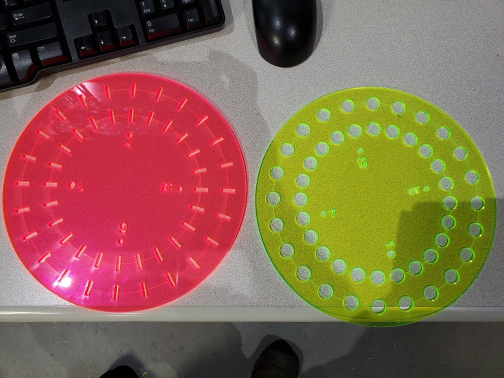
Fig. 8.2 Double-ring sample wheels with 48 sample positions. There are options for both wheel styles with 13mm x 3 mm slots or 13mm diameter holes. The rings on the double wheel are 26 mm apart (center to center of slots/holes).

The automation concept is that each slot on the sample wheel is described by a row in the spreadsheet. Each column of the spreadsheet carries one parameter of the XAFS scan.

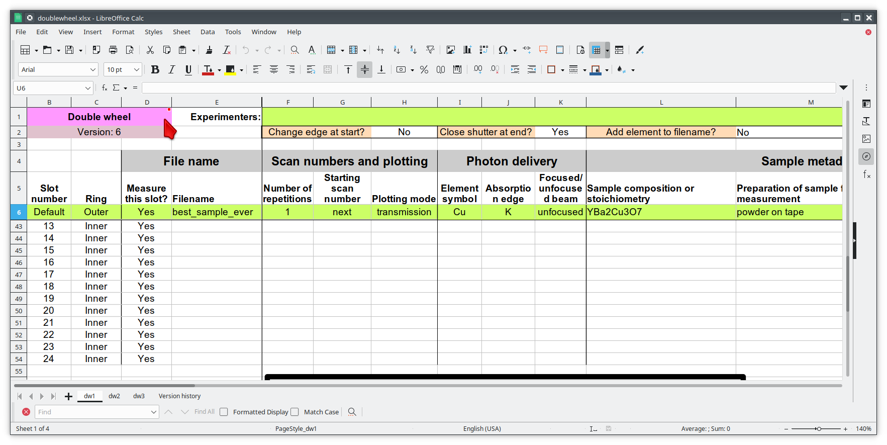
Fig. 8.3 Example spreadsheet for running an experiment from a wheel with a two sample rings. Links: single wheel spreadsheet and double wheel spreadsheet.

If you have read Section 7.1 about the INI file, then most of the columns in this spreadsheet will be quite familiar. Most of the columns are used to specify the same set of parameters as in the INI file – file name, element, edge, and so on.

The green cell in the first row is used to input the names of all the people involved in the experiment, as explained above.

As explained above, row 6, row with an entirely green background, is used to specify the default values for all the parameters. The concept here is to try to avoid having to input repetitive information. For instance, in this case, all measurements will be made at the Fe K edge. The element and edge are all specified in the green row. Those cells are left blank for all subsequent rows, so the default values will be used.

In short, any cell that is left blank will use the value from the green, default row. Any cell for which a value is specified will be used in the macro that gets generated.

The first column is used to specify the slot number for each sample on the sample wheel.

The second column is a simple way of excluding the slot from measurement simply by specifying No.

The next several columns correspond to lines in the INI file as explained in Section 7.1.

Energy changes can be included in the macro by specifying different values for element and/or edge in a row. When specified and different from the previous row, a call to the change_edge() command (Section 5) is inserted into the macro.

Not shown in Figure 8.1 are columns for tweaking the xafs_x and xafs_y positions, adjusting the horizontal and vertical size of slits3 (see Section 5.6), and adjusting the fluorescence detector position.

Again, assuming the tab in the spreadsheet was called mysamples, you can then run the macro generated from the spreadsheet by:

RE(mysamples_macro())

Here are the first few lines of the macro generated from this spreadsheet. Note that for each sample, the macro first moves using the slot() command, then measures XAS using the xafs() command. The xafs() command uses the INI file (Section 7.1) generated from the green default line and has explicit arguments for the filled-in spreadsheet cells.

yield from slot(1)
yield from xafs('MnFewheel.ini', filename='Fe-Rhodonite', sample='MnSiO3', comment='ID:93 Russia')
close_last_plot()

yield from slot(2)
yield from xafs('MnFewheel.ini', filename='Fe-Johannsonite', sample='CaMnSi2O6 - LT', comment='B –Iron Cap Mine; Graham Country, Arizona')
close_last_plot()

yield from slot(3)
yield from xafs('MnFewheel.ini', filename='Fe-Spessartine', sample='Mn3Al2(SiO4)3', comment='Grants Mining District; New Mexico')
close_last_plot()

8.3. Linkam stage automation

One of the temperature control options at BMM is a Linkam stage. Ours is the kind that can cool using liquid nitrogen flow or heat up to 600 C using a resistive heater. The linkam stage is typically mounted upright on top fo the XY stage.

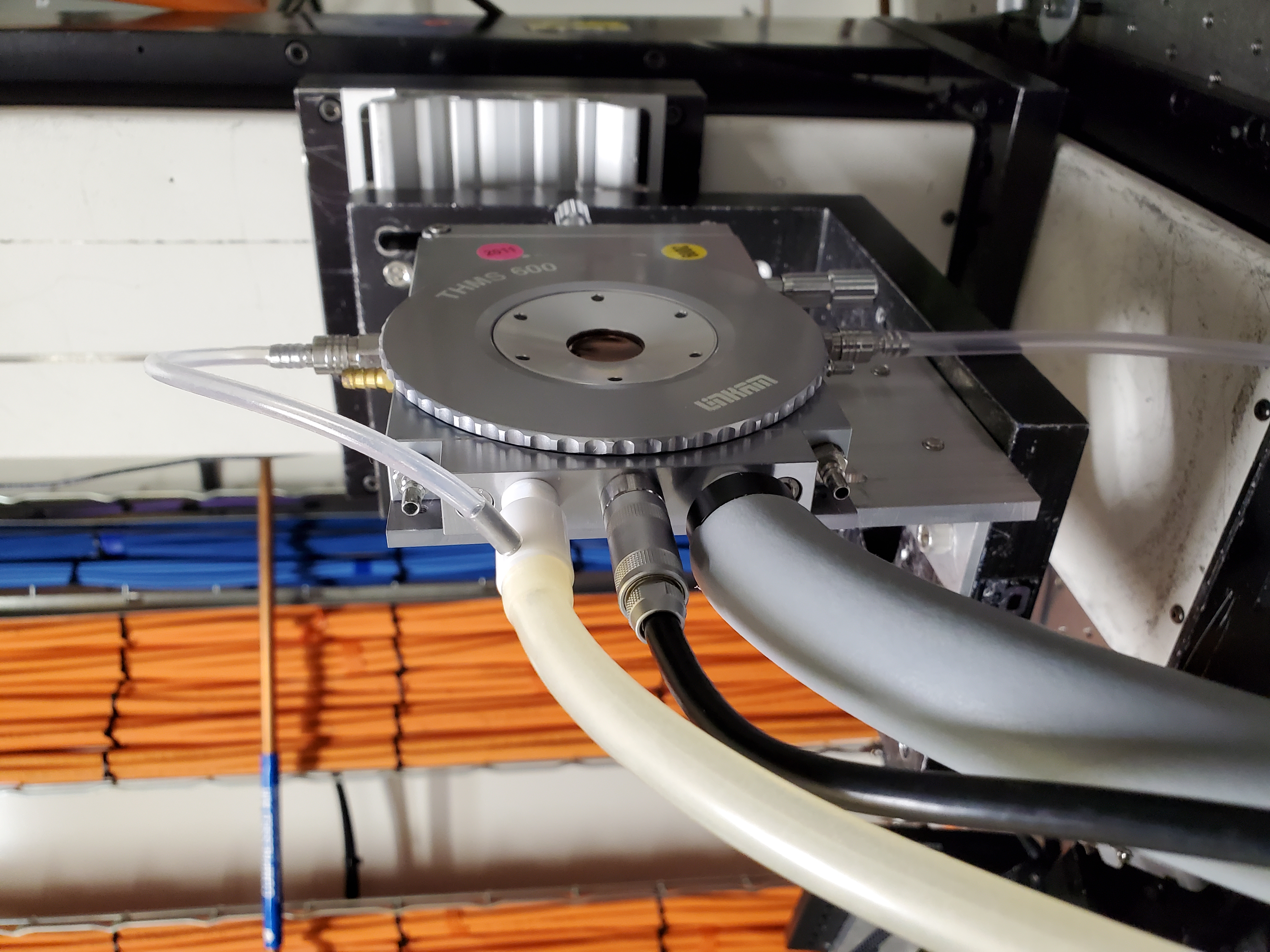
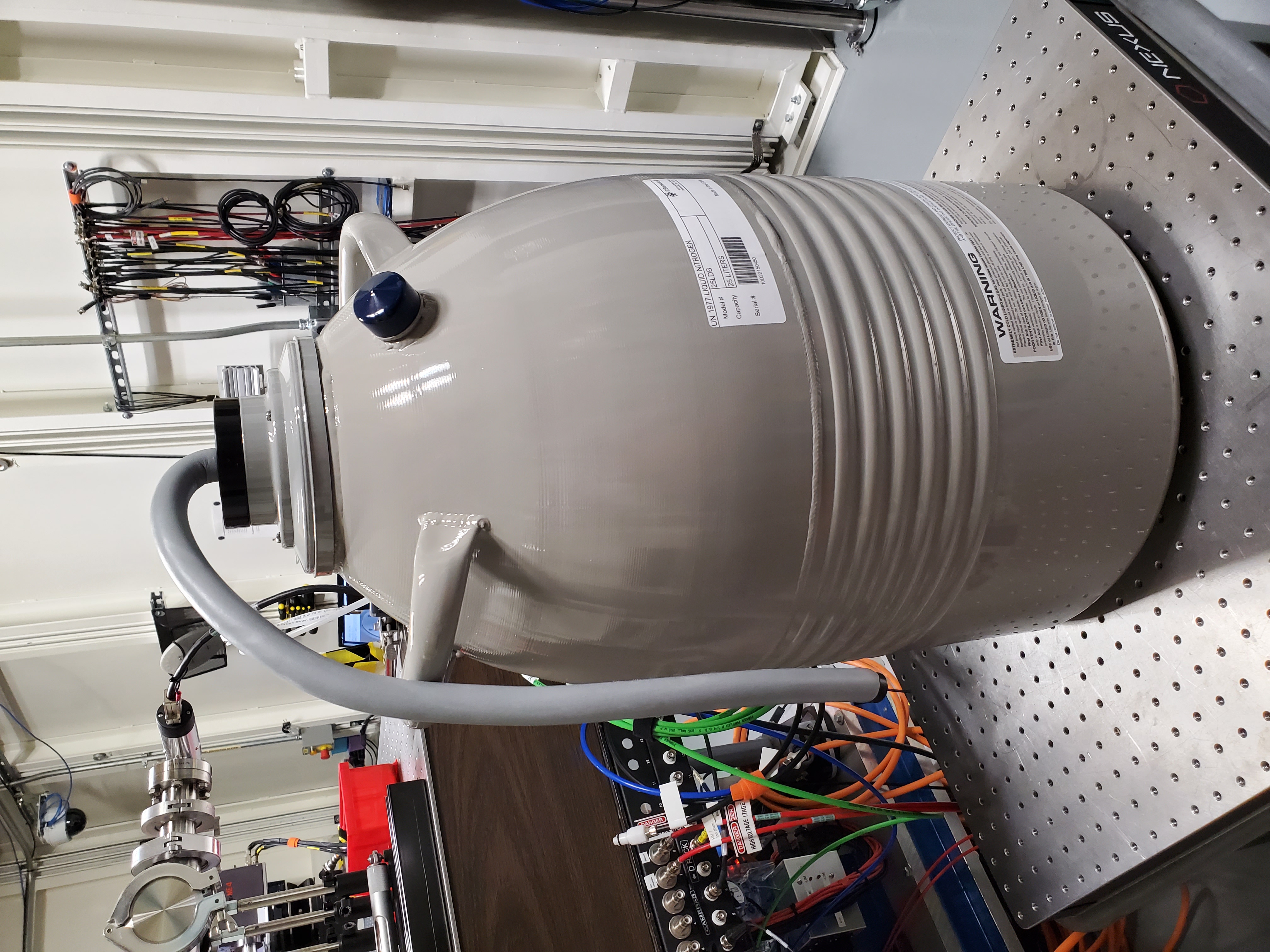
Fig. 8.4 (Left) The Linkham stage mounted for transmission on the sample stage. (Right) The 25 L dewar used for cooling the Linkam stage.

The automation concept for the Linkam stage is quite similar to the ex situ sample holder. Instead of specifying the slot position of the sample, you will specify the target temperature for the measurement. There is also a column for specifying the holding time after arriving at temperature before beginning the XAFS measurement.

The feature described in Section 8.1.3 for modifying filenames is particularly useful in this context. It can be used to put the measurement temperature in the filename, allowing you to simply specify a default filename, leaving that cell in each row blank. The generated data files will then have sensible names.

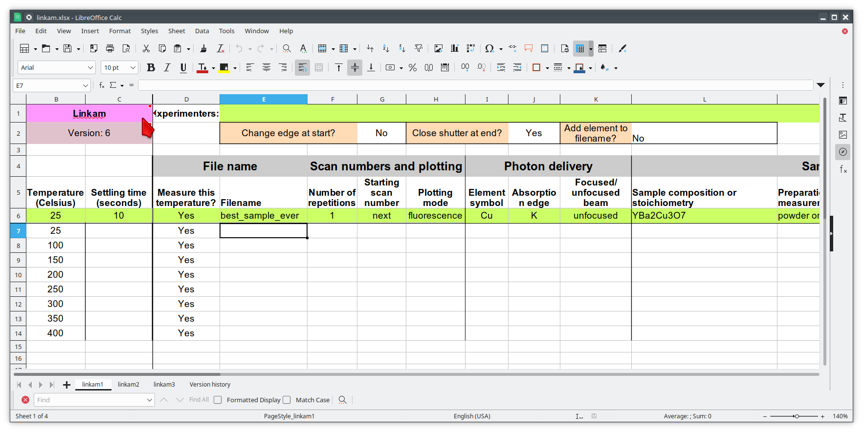
Fig. 8.5 Example spreadsheet for running a temperature-dependent experiment using the Linkam stage. Link to the Linkam spreadsheet

8.4. LakeShore/Displex automation

For extremely low temperature experiments, BMM has a Displex crystat which uses a two-stage helium compressor to cool the cold head down as low as 10K with temperature control between 10K and 500K using a resistive heater and a LakeShore temperature controller.

This is a somewhat unusual version of the Displex system in that it is suitable for low-vibration applications. The compressor is mechanically decoupled from the cold head, reducing the motion of the sample. As a result of this cooling system, it is somewhat time-consuming to temperature cycle and replace samples. Expect that cooling from room temperature to 10K will take about 2 hours and budget up to an an hour for returning to room temperature and changing samples.

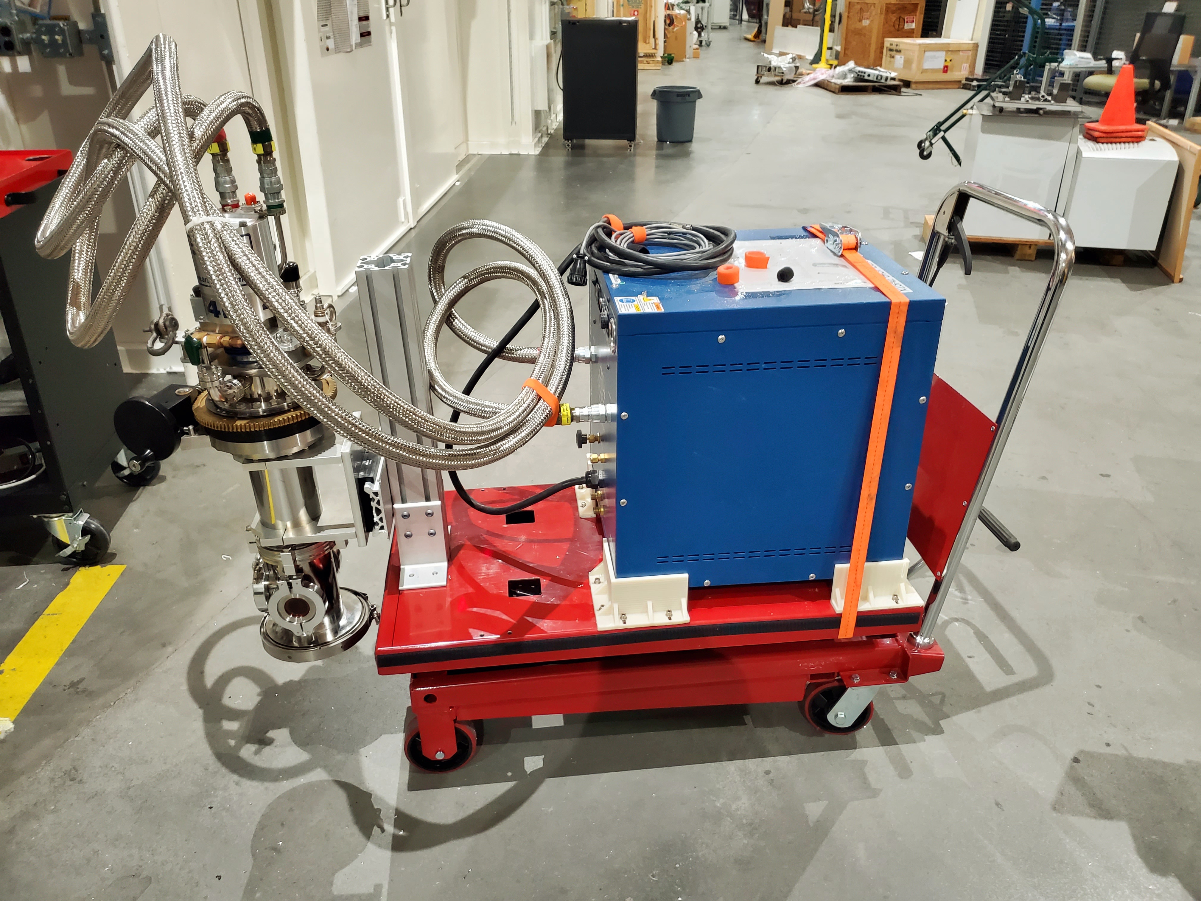
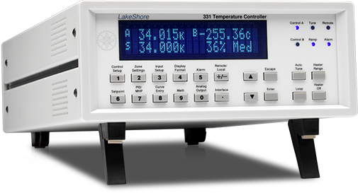
Fig. 8.6 (Left) The Displex cryostat and it’s compressor. (Right) The LakeShore 331 controller, used to control temperature for the cryostat shown to the left.

The automation for the LakeShore 331 works much the same as for the Linkam stage. Again, you will specify the target temperature for the measurement. And there is a column for specifying the holding time after arriving at temperature before beginning the XAFS measurement.

There is a column for specifying the power level of the heater in the cryostat. There are three power settings.

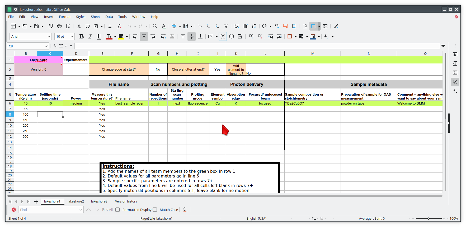
Fig. 8.7 Example spreadsheet for running a temperature-dependent experiment using the Displex cryostat and the LakeShore 331. Link to the LakeShore spreadsheet.

8.5. Glancing angle stage automation

This stage is used to automate measurement at glancing angle, usually on thin film samples. The stage can be mounted horizontally or vertically, allowing measurement of in- or out-of-plane strain in thin films.

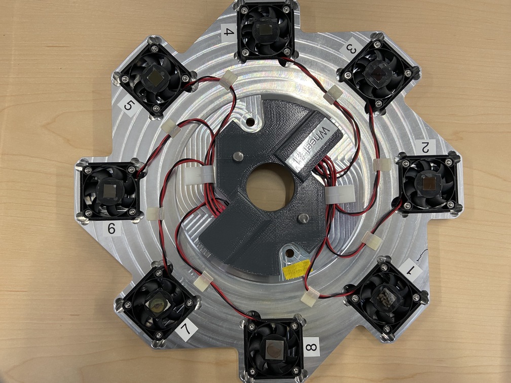
Fig. 8.8 The glancing angle stage with 8 sample positions.

This stage is mounted on a rotation stage to move between samples. The rotation stage is mounted on a tilt stage to set the incident angle of the beam relative to the sample surface. This entire set up is mounted on the XY stage for alignment on the beam.

Each sample is affixed to a sample spinner (which is simply a cheap, 24 VDC CPU fan). The 8 spinners are independently controlled via slip ring electrical connection that runs through the axis of the rotation stage. In practice, only the sample that is being measured is spinning.

Again, the automation concept is very similar to the ex situ sample wheel. Instead of specifying slot number, the spinner number is specified on each row. There is also a yes/no menu for specifying whether the sample spins during measurement.

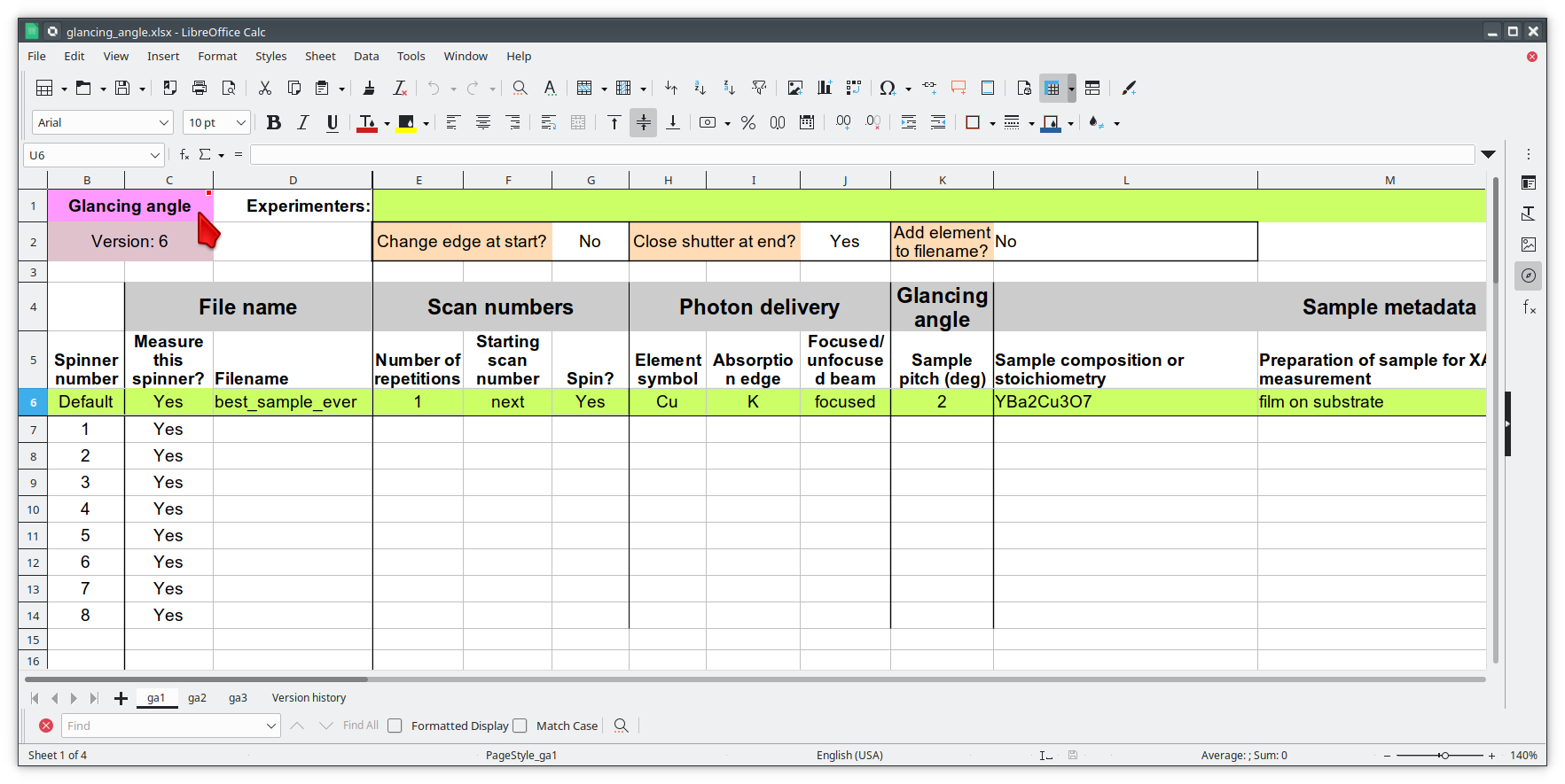
Fig. 8.9 Example spreadsheet for running an experiment using the glancing angle stage. Link to the glancing angle spreadsheet.

Not shown in Figure 8.9 are columns for specifying how sample alignment is handled. The default is to do automated alignment. This works by following this script:

1. Move the stage to an incident angle that is close to flat for the sample and start the sample spinning.

2. Do a scan in the vertical direction, measuring the signal in the transmission chamber. Fit an error function to the transmission signal. The centroid of that function is the position with the sample half-way in the beam.

3. Do a scan in pitch, measuring the signal in the transmission chamber. The peak of that measurement is the position where the sample is flat relative to the beam direction.

4. Repeat steps 2 and 3.

5. Move the sample tilt to the angle specified by the user in the spreadsheet.

6. Do a scan in the vertical direction, measuring the signal in the fluorescence detector. The center of mass of that measurement is the position where the beam is well-centered on the sample.

The result of this fully automated sequence is shown in Figure 8.10.

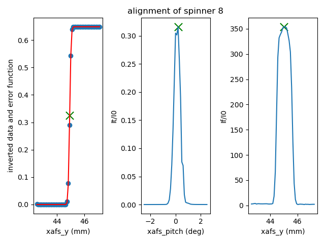
Fig. 8.10 This visual representation of the automated glancing angle alignment is posted to Slack and presented in the measurement dossier (Section 9.4).

For some samples, the automated alignment is unreliable, so there is an option in the spreadsheet for manual alignment. In that case, find the xafs_y and xafs_pitch positions for the sample at its measurement angle and well-aligned in the beam. Enter those numbers and they will be used by the macro rather than performing the automated alignment.

8.6. Motor grid automation

The final kind of automation-via-spreadsheet available is BMM is for a generic motor grid. The most common motor grid used for measurement is the sample XY stage, xafs_x and xafs_y. However, any two motors on the beamline can be used for the grid.

There are columns (to the left of the view shown in Figure 8.11) for specifying the axes in the grid.

In all other ways – except for the slot column – this spreadsheet is identical to the ex situ sample wheel spreadsheet.

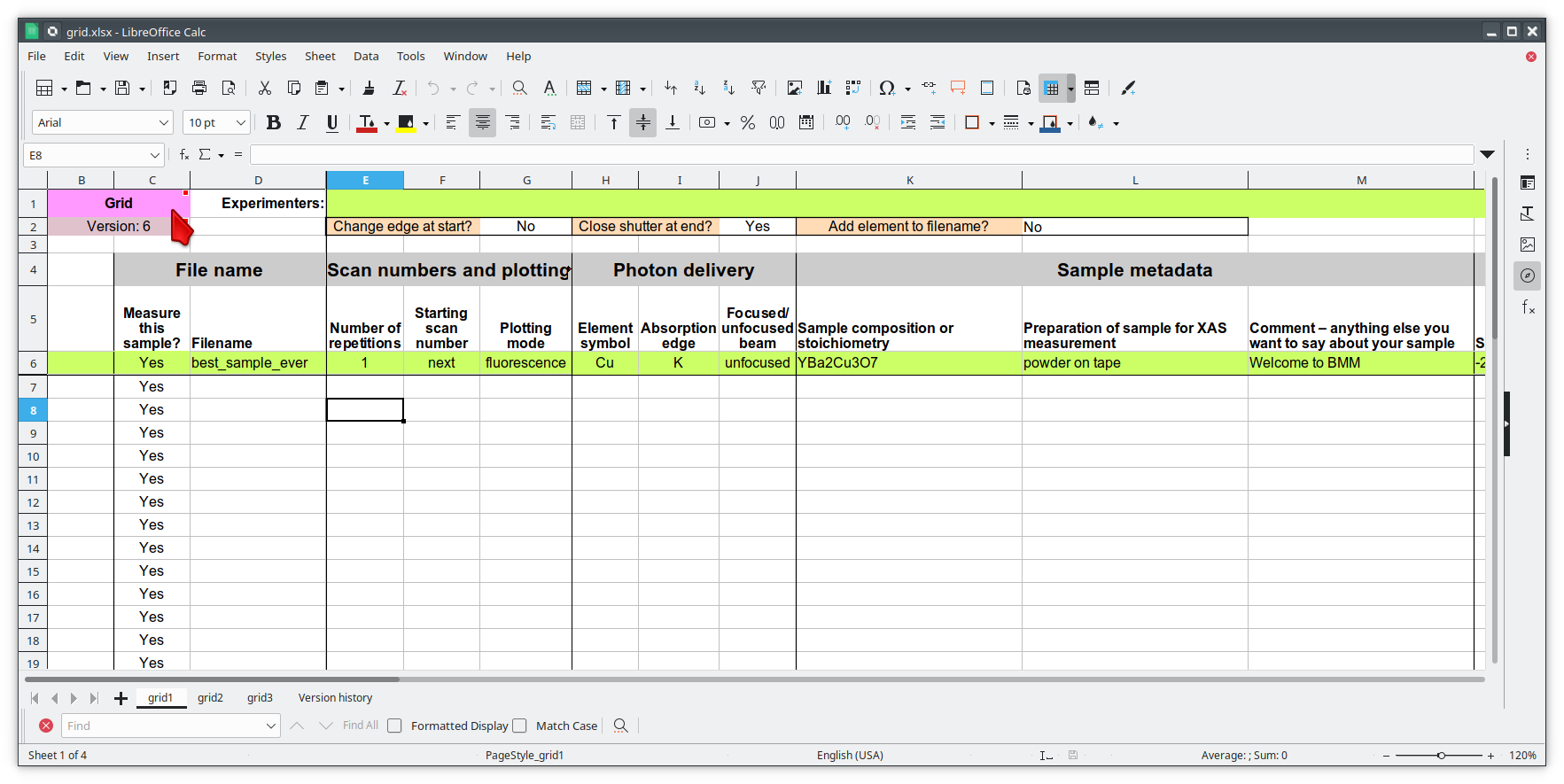
Fig. 8.11 Example spreadsheet for running an experiment on an XY grid. Link to the motor grid spreadsheet.

Caution

Spreadsheets with version number earlier 13 will not work as of 1 March, 2024.