
7. Photon Delivery System#
7.1. Overview#
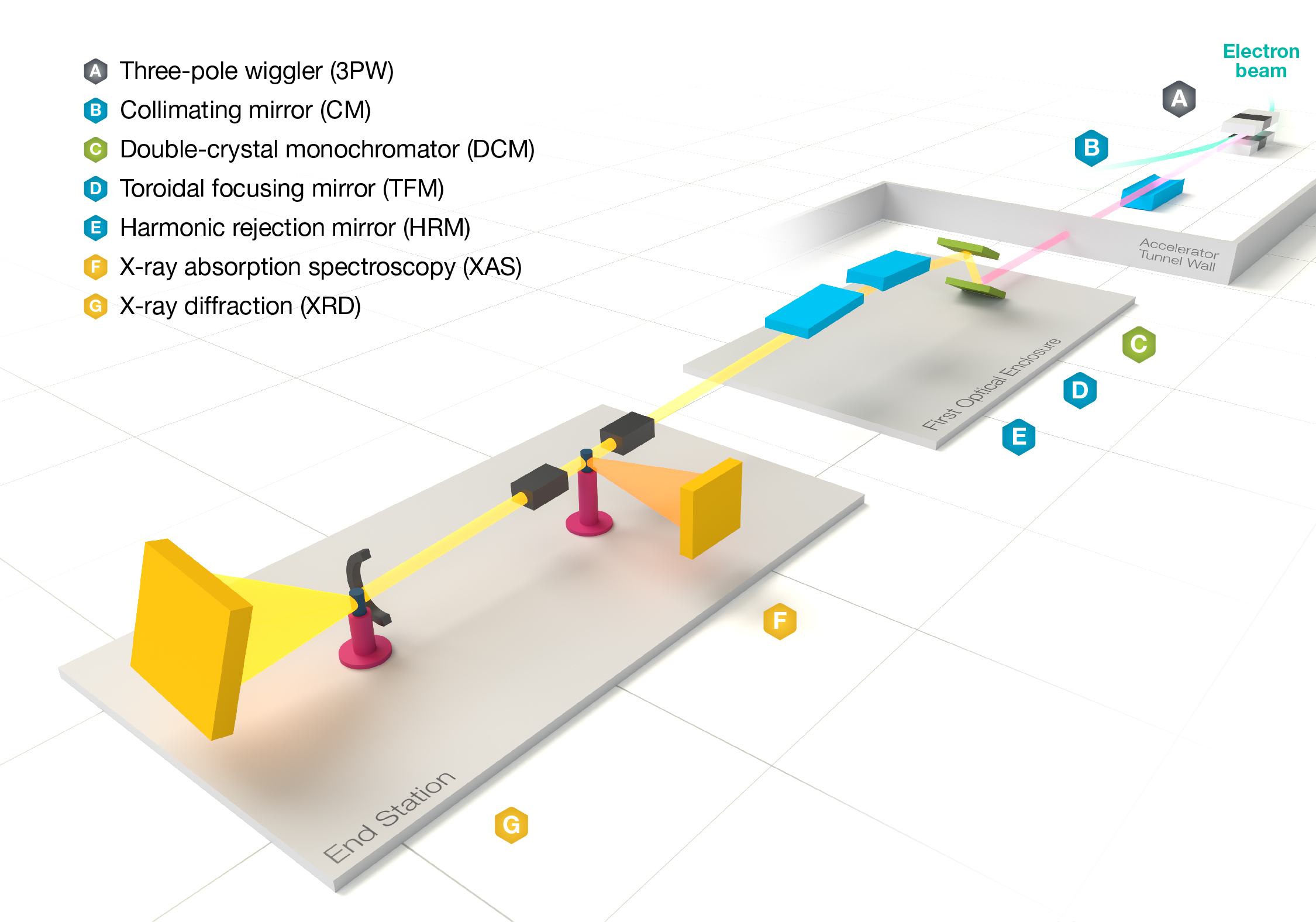
Fig. 7.1 Beamline optics layout for BMM. Thanks to Tiffany Bowman for this lovely beamline schematic.#
- Source
The source at BMM is an NSLS-II three-pole wiggler (TPW). (See Section G.4 for some photos of the source device.) This device has a spectrum that resembles a bending magnet, but shifted to higher energy compared to the NSLS-II bending magnet.
- Collimating Mirror
The first optical component is a paraboloid collimating mirror. This device is 5 nm of Rh on 30 nm of Pt on a silicon substrate. This fixed-angle, fixed-figure device corrects the dispersion of the TPW source and directs the collimated beam toward the ratchet wall aperture.
Danger
There is never a reason to move the first mirror. It is in the correct orientation for collimation and delivery of beam through the ratchet wall.
Moving any first mirror motor runs the risk of leaving the first mirror in a non-functional state!
- Monochromator
The collimated beam then hits the double crystal monochromator (DCM). BMM has pairs of Si(111) and Si(311) crystals, accessibly by lateral translation of the DCM vacuum vessel. This is a fixed-exit monochromator which moves the second crystal parallel and perpendicular to the crystal surfaces to direct the monochromatic beam towards a small aperture in the pink beam mask and Bremsstrahlung shield.
- Focusing and harmonic rejection mirrors
Downstream of the monochromator are a torroidal focusing mirror (TFM) and a flat harmonic rejection mirror (HRM). The TFM is coated with 5 nm of Rh on 30 nm of Pt. The HRM has a Rh/Pt stripe and a bare silicon stripe. The bare silicon stripe is used below 8 keV for improved harmonic rejection.
The angle and bend of the TFM can be adjusted to deliver focused beam either to the XAS end station or to the center of the goniometer.
At high energies, either the TFM or the HRM is in the beam path. At low energies, the HRM or both mirrors are in use. See Section 7.8.1 for details of the mirror configuration modes.
See MA Marcus, et al., J. Synch. Radiat. (2004) 11, 239-247 for an explanation of the Pt/Rh coating scheme.
7.2. Configure for an Absorption Edge#
Configuring the photon delivery system for a specific measurement is usually quite simple. When moving to a new absorption edge, do the following:
RE(change_edge('Fe'))
substituting the two-letter symbol for the element you want to measure. This will:
move the monochromator (Section 7.4)
put the photon delivery system in the correct mode (Section 7.8.1)
measure the rocking curve of the monochromator (Section 8.2)
optimize the height of the hutch slits (Section 8.2)
move the reference foil holder to the correct position (Section 6.1)
set the active Xspress3 ROI to the correct emission line
This whole process takes at most 7 minutes, sometimes under 3 minutes. After that, the beamline is ready to collect data.
If using the focusing mirror, do this:
RE(change_edge('Fe', focus=True))
Excluding the focus argument – or setting it to False –
indicates setup for collimated beam.
This edge change can be put into a macro (see Section 9.6) like so:
yield from change_edge('Fe')
or
yield from change_edge('Fe', focus=True)
In this way, a macro can manage energy changes while you sleep!
7.2.1. Automating reference foil changes#
A wheel is used to hold and switch between reference foils and stable oxides. The standard reference wheel has most of the elements accessible at BMM, including all the lanthanides (except Pm!). A double wheel (see Figure 11.2) is used to hold the standards. The wheel is mounted on a rotation stage which is, in turn, mounted on an XY stage for alignment. See Table 9.2 for the contents of reference wheel.
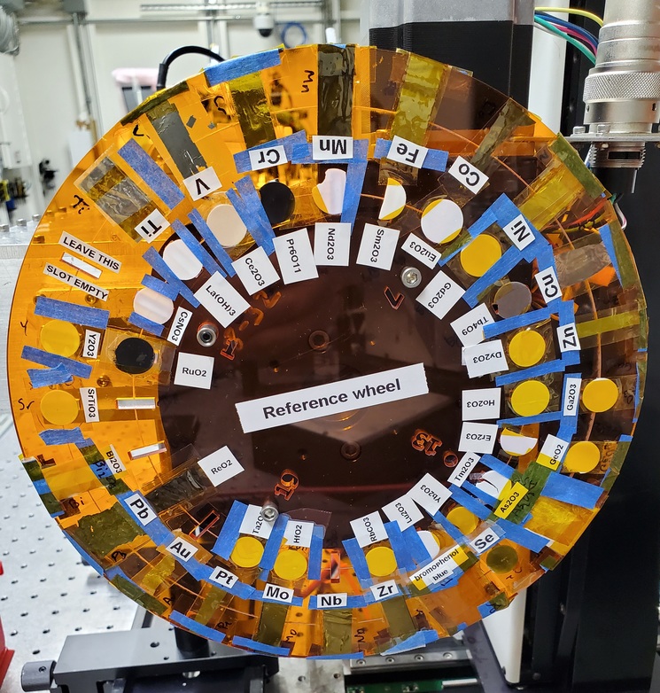
Fig. 7.2 The reference wheel.#
To select, for example, the iron reference foil:
RE(reference('Fe'))
In a plan:
yield from reference('Fe')
The argument is simply the one- or two-element symbol for the target element.
This selects the correct reference by rotating to the correct slot and translating to the correct ring on the wheel.
The change_edge() command does this automatically, so long as the
target edge is available on the reference holder.
The reference wheel content is configured as a python dictionary. See
xafs_ref.mapping, defined here.
This dictionary identifies the positions in xafs_ref and
xafs_refx for each reference sample. It also identifies the form
of the reference samples and its chemical composition.
To see the available reference materials and their positions on the
reference wheel, do %se.
Here is a complete list of standards in BMM’s collection.
7.2.2. Parameters for the change_edge() command#
Typically the change_edge() command is called with one or two
arguments, the mandatory element symbol and the the focus
argument, which can be True or False.
The full set of parameters for the change_edge() plan are:
RE(change_edge(element, focus=False, edge='K', energy=None, tune=True, slits=True, calibrating=False, target=300.))
where,
elementThe one- or two-letter element symbol or Z number.
focusTrue: set up for using the focusing mirror, modes A, B, C;False: collimated beam, modes D, E, F. Default isFalse.edgeIf not specified, use K or L3, as appropriate for the energy range of the beamline. Use this argument to specify an L1, L2, or M edge.
energyUse an E0 value that is not obtained from the look-up table. Default is unspecified, i.e. use
elementand look-up table. This is rarely necessary, except when setting up for XRD (Section 13.4).insistTrue: Force movement of M2 motors;False: decide normally whether to move M2 motors. Default isFalse.tuneTrue: optimize DCM second crystal pitch;False: skiprocking_curve()scan. Default isTrue. Skipping this is rarely a good idea.slitsTrue: optimize slit height;False: skipslit_hight()scan. Default isTrue. Skipping this is rarely a good idea.no_refTrue: skip moving to the correct reference foil. Default isFalse. Used when the reference stages have been repurposed for other use in an experiment.calibratingTrue: used when performing beamline maintenance. Default isFalse. Rarely used.targetThe energy above e0 at which to perform the rocking curve scan. Default is 300. Care is taken not to exceed an L2 edge energy (or L1 when measuring L2).
Except for edge and focus, most of those parameters are rarely
used. If you need to measure an L2 or L1 edge, you
must specify edge. For example:
RE(change_edge('Pt', edge='L1'))
For all the details about the individual parts of the photon delivery system, read on!
7.3. Shutters#
- Open and close the photon shutter
In the nomenclature of BMM, the photon shutter is
shb. Open and close this shutter with:shb.open() shb.close()
These plans are somewhat more elaborate than simply toggling the state of the shutters. It happens from time to time that the shutter does not trigger when told to open or close. So, these plans try up to three times to open or close the photon shutter, with a 1.5 second pause between attempts.
If you wish to open or close the photon shutter (using the same multiple attempt algorithm) in a macro (Section 9.6), do:
yield from shb.open_plan()
yield from shb.close_plan()
- Open and close the safety shutter
This is the front-end shutter. Closing it takes light off the monochromator, which is not something you typically want to do during an experiment. That said, the safety shutter is
shain the BMM nomenclature:sha.open() sha.close()
and:
yield from sha.open_plan()
yield from sha.close_plan()
7.4. Monochromator#
The monochromator consists of 8 motors. It should never be necessary to interact directly with any of the physical motors. Plans exist for facilitating any actions a user should ever need.
- Query the current energy
To know the position and energy of the monochromator:
%w dcmThis returns a short report like this:
Energy = 19300.1   reflection = Si(111)
current: Bragg =  5.87946   2nd Xtal Perp = 15.0792   2nd Xtal Para = 146.4328
This report shows the current energy, the crystal set currently in use, and the position of the parallel and perpendicular motors of the second crystal carriage.
- Move to a new energy
The
dcm.energyvirtual motor coordinates the Bragg, parallel, and perpendicular motors to maintain a fixed exit height and set the energy of the mono. To move to the copper K edge energy:RE(mv(dcm.energy, 8979))
To move 50 eV above the copper K edge energy:
RE(mv(dcm.energy, 8979+50))
Note that the BlueSky command line is able to do simple arithmetic (and a whole lot more!). It is a good idea to leave the arithmetic to the computer.
- Move to a new energy in a macro
An energy change can be a part of a macro (Section 9.6). Simply do:
yield from mv(dcm.energy, 8979+50))
- Tune the second crystal of the mono
After a long move, you might need to retune the second crystal. To find the peak of the rocking curve and move to that peak:
RE(rocking_curve())
This will run a scan of the pitch of the second crystal. At the end of the scan, it moves to the center of mass of the measured intensity profile.
You can do the rocking curve scan by looking at the signal on the Bicron which is used as the incident beam monitor for the XRD end station. Do:
RE(rocking_curve(detector='Bicron'))
You can tune the second crystal by hand with these commands:
tu()
td()
Those stand for “tune up” and “tune down”. Do not think that “up” and “down” refer to measured intensity. Rather, they refer to the direction of motion of the motor which adjusts the second crystal pitch. When you move to higher energy, you usually need to tune in
td()direction. When you move to a lower energy, you usually need to tune in thetu()direction. Obviously…..- Fixed-exit and pseudo-channelcut modes
The mono can be run in either fixed-exit or pseudo-channelcut modes.
Fixed exit means that the second monochromator crystal will be moved in directions parallel and perpendicular to its diffracting surface in order to maintain a fixed exit height of the beam coming from the second crystal. Without fixed-exit mode, it would not be possible to change the energy over the entire energy range of the beamline. The aperture after the monochromator is only a few millimeters tall. The vertical displacement of the beam over a lerge energy change would be sufficient to move the beam out of the aperture.
However, the stability of the monochromator suffers with respect to EXAFS data quality when measuring an energy scan in fixed-exit mode. We find it is better to disable the parallel and perpendicular motions when measuring XAFS, suffering a small vertical displacement of the beam.
The mono mode is controlled by a parameter:
dcm.mode = 'fixed'
or
dcm.mode = 'channelcut'
In practice, the monochromator is normally left in fixed-exit mode. That way, the monochromator can be moved without having to worry about the beam height and the monochromator exit aperture. In the XAFS scan plan (Section 9.4), the monochromator first moves – in fixed-exit mode – to the center of the angular range of the scan, then sets
dcm.modetochannelcut. Once the sequence of scan repititions is finished, the monochromator is moved back to the center of the angular range and the monochromator is returned to fixed-exit mode.
7.5. Post-mono slits#
After the mono, before the focusing mirror, in Diagnostic Module 2, there is a four-blade slit system. These are used to define the beam size on the mirrors and to refine energy resolution for the focused beam.
The typical size of the post-mono slits is 18 mm in the horizontal and 1.3 mm in the vertical.
motor |
units |
notes |
motion type |
|---|---|---|---|
slits2_top |
mm |
top blade position |
single axis |
slits2_bottom |
mm |
bottom blade position |
single axis |
slits2_inboard |
mm |
inboard blade position |
single axis |
slits2_outboard |
mm |
outboard blade position |
single axis |
slits2_hsize |
mm |
horizontal size |
coordinated motion |
slits2_hcenter |
mm |
horizontal center |
coordinated motion |
slits2_vsize |
mm |
vertical size |
coordinated motion |
slits2_vcenter |
mm |
vertical center |
coordinated motion |
The individual blades are moved like any other motor:
RE(mv(slits2.outboard, -0.5))
RE(mvr(slits2.top, -0.1))
Coordinated motions are moved the same way:
RE(mv(slits2.hsize, 6))
RE(mvr(slits2.vcenter, -0.1))
To know the current positions of the slit blades and their coordinated
motions, use %w slits2
In [1966]: %w slits2
SLITS2:
     vertical   size   =   1.350 mm          Top      =   0.675
     vertical   center =   0.000 mm          Bottom   =  -0.675
     horizontal size   =   8.000 mm          Outboard =   4.000
     horizontal center =   0.000 mm          Inboard  =  -4.000
7.6. Mirrors#
Mirrors are set as part of the mode changing plan. Unless you know
exactly what you are doing, you probably don’t want to move the
mirrors outside of the change_mode() command. (Adjusting M1 by
hand is a horrible idea – unless you know exactly what you are doing
and why.) Changing the mirror positions in any way changes the height
and inclination of the beam as it enters the end station. This
requires changes in positions of the slits, the XAFS table, and other
parts of the photon delivery system.
Outside of the use of the change_mode() command, it should not be
necessary for users to move the mirror motors. It is very easy to
lose the beam entirely when moving mirror motors. Without a clear
understanding of how the optics work, re-finding the beam can be quite
challenging.
Attention
If you loose the beam by moving mirror motors, the
easiest solution is to rerun the change_mode() command,
possibly with the insist=True argument.
If you want to know the current positions of the motors on the
focusing mirror, use %w m2
In [1903]: %w m2
M2:
     vertical =   6.000 mm           YU  =   6.000
     lateral  =   0.000 mm           YDO =   6.000
     pitch    =   0.000 mrad         YDI =   6.000
     roll     =  -0.001 mrad         XU  =  -0.129
     yaw      =   0.200 mrad         XD  =   0.129
     bender   =  163789.0 steps
For the harmonic rejection mirror, use %w m3
In [1904]: %w m3
M3: (Rh/Pt stripe)
     vertical =   0.000 mm           YU  =  -1.167
     lateral  =  15.001 mm           YDO =   1.167
     pitch    =   3.500 mrad         YDI =   1.167
     roll     =   0.000 mrad         XU  =  15.001
     yaw      =   0.001 mrad         XD  =  15.001
The front-end collimating mirror, the focusing mirror, and one stripe of the harmonic rejection mirror are coated with 5 nm of Rh deposited on 30 nm of Pt on silicon. See MA Marcus, et al., J. Synch. Radiat. (2004) 11, 239-247 DOI: 10.1107/S0909049504005837 for an explanation of the advantages of this coating scheme.
7.7. End station slits#
Near the end of the photon delivery system, in Diagnostic Module 3 in the end station, there is a four-blade slit system. These are used to define the beam size on the sample.
motor |
units |
notes |
motion type |
|---|---|---|---|
slits3_top |
mm |
top blade position |
single axis |
slits3_bottom |
mm |
bottom blade position |
single axis |
slits3_inboard |
mm |
inboard blade position |
single axis |
slits3_outboard |
mm |
outboard blade position |
single axis |
slits3_hsize |
mm |
horizontal size |
coordinated motion |
slits3_hcenter |
mm |
horizontal center |
coordinated motion |
slits3_vsize |
mm |
vertical size |
coordinated motion |
slits3_vcenter |
mm |
vertical center |
coordinated motion |
The individual blades are moved like any other motor, for example:
RE(mv(slits3.outboard, -0.5))
RE(mvr(slits3.top, -0.1))
Coordinated motions are moved the same way, for example:
RE(mv(slits3.hsize, 6))
RE(mvr(slits3.vcenter, -0.1))
To know the current positions of the slit blades and their coordinated
motions, use %w slits3
In [1966]: %w slits3
SLITS3:
     vertical   size   =   1.350 mm          Top      =   0.675
     vertical   center =   0.000 mm          Bottom   =  -0.675
     horizontal size   =   8.000 mm          Outboard =   4.000
     horizontal center =   0.000 mm          Inboard  =  -4.000
7.8. Configurations#
7.8.1. Photon delivery modes#
A look-up table is used to move the elements of the photon delivery system to their correct locations for the different energy ranges and focusing conditions. Here is a table of different photon delivery modes. Modes A-F are for delivery of light to the XAS end station. Mode XRD delivers high energy, focused beam to the goniometer.
Mode |
focused |
energy range |
|---|---|---|
A |
✓ |
above 8 keV |
B |
✓ |
below 6 keV |
C |
✓ |
6 keV – 8 keV |
D |
✗ |
above 8 keV |
E |
✗ |
6 keV – 8 keV |
F |
✗ |
below 6 keV |
XRD |
✓ |
above 8 keV |
Todo
The lookup table is not complete for mode B. In fact, the ydo and ydi jacks of M3 cannot move low enough to enter mode B. In practice, mode B is not available. Elements that should be measured in mode B are, instead, measured in mode C and we live with incomplete harmonic rejection.
To move between modes, do:
RE(change_mode('<mode>'))
where <mode> is one of the strings in the first column of
Table 7.3. For example:
RE(change_mode('D'))
This will move 17 motors all at the same time and should take less than 5 minutes.
Focusing at the XAS end station requires that bender be near its upper limit. Focusing at the XRD station has the bender near the middle of its range.
7.8.2. Monochromator crystals#
To change between the Si(111) and Si(311) crystals, do:
RE(change_xtals('111'))
or:
RE(change_xtals('311'))
This will move the lateral motor of the monochromator between the two crystal sets and adjust the pitch of the second crystal to be nearly in tune and the roll to deliver the beam to nearly the same location for both crystals. It will also return the monochromator to the starting energy.
This takes about 5 minutes.
The change_xtals() plan also runs the rocking curve
(Section 8.2) macro to fix the tuning of the
second crystal.