9. XAFS scans#
The simplest access to an XAFS scan starts by editing an INI file. This is a simple keyword/value system where the keyword is separated from the value by an equals sign and each line contains a single keyword/value pair.
This file captures the set of metadata that the user supplies to specify the details of the step scan, the basic configuration of the beamline, and some details about the sample preparation. Most of this metadata is captured in the beamline database and written to the header of the output data files.
This file is typically stored in the same folder where the data files are written and is called by name when running an XAFS scan.
Note that the concepts and language used in the INI file is repeated throughout the spreadsheets used for beamline automation (Section 11).
9.1. The INI file#
 1[scan]
 2filename      = cufoil
 3experimenters = Betty Cooper, Veronica Lodge, Archibald Andrews
 4
 5element    = Cu
 6edge       = K
 7sample     = Cu metal
 8prep       = standard foil
 9comment    = Welcome to BMM
10
11nscans     = 3
12start      = next
13
14# mode is transmission, fluorescence, both, or reference
15mode       = transmission
16
17##  regions relative
18##  to e0:         1      2      3      4
19bounds     = -200    -30     -10   15.5    15k
20steps      =      10     2.0    0.3    0.05k
21times      =      0.5    0.5    0.5    0.25k
Here is a complete explanation of the contents of the INI file.
filename(line 2)The stub for the names of the output data files and the snapshots. In the example above, the files written disk will be called
cufoil.001,cufoil.002, and so on.experimenters(line 3)The name of the participants in the measurement. Because all data and metadata reside in a database, specifying experimenter names makes it easy to search the database for data associated with a specific person.
element(line 5)The one- or two-letter symbol for the element. The edge energy,
e0, will be looked up usingelementandedge.edge(line 6)The symbol (
K,L3,L2,L1) of the edge being measured.sample(line 7)This is intended to capture the stoichiometry or composition of the sample being measured.
prep(line 8)This is intended to capture the details of how the sample was prepared for the XAFS measurement.
comment(line 9)This is for anything else you might want to say about your sample.
nscansandstart(lines 11 - 12)These are used to form the file extension of the output data file. They indicate the starting value of the number used as the file extension and how many repetitions of the scan to make. The file extension is always a zero-padded, three-digit number, e.g.
cufoil.001,cufoil.002, and so on.The most common value for this parameters is the word
next, in which case thefolderwill be searched for files starting withfilenameand ending in a number. The subsequent number will be used. E.g. ifcuedge.007is the highest numbered file in thecuedgesequence, running XAFS again using the same INI file will start withcuedge.008.startcan also be a positive integer, in which case it will be the first number used in the sequence of scans. So if the value is 137, the first file will be calledcufoil.137.mode(line 15)Indicate how data should be displayed on screen during a scan. The options are
transmission,fluorescence,both, orreference.bothmeans to display both the transmission and fluorescence during the scan.This parameter also controls what gets written to the output data files. In all cases, the signals from I0, It, and Ir are written to the data file. If
modeisfluorescenceorboth, then 4 columns related to the fluorescence detector are also written. The columns are labeled something likeCu1,Cu2,Cu3, andCu4(whereCuwould be replaced by the symbol of the element
Comments begin with the hash (#) character and are ignored.
9.1.1. Scan regions#
In a typical step scan, we measure data on a coarse grid in the
pre-edge, a fine grid through the edge region, and on a constant grid
in photoelectron wavenumber in the extended region. The bounds,
steps, and times keywords (lines 19-21) are used to set this
grid.
bounds indicates the energies – relative to the e0 value
– where the step sizes and dwell times will change. There must
always be one more value in the bounds list than in the steps
and times lists.
For the bounds and steps lists, values must be either a
number or a string consisting of a number followed by the letter
k. Numbers followed by k are interpreted as being values in
photoelectron wavenumber and are only sensible above the edge.
You may switch back and forth between energy and wavenumber values.
The bounds and steps lists are converted to energy values
before being used.
In the bounds lists, an energy value indicates an energy below or
above the e0 value. A wavenumber value inidcates a wavenumber
value above the edge.
In the steps list, an energy value indicates a step size in eV. A
wavenumber value indicates a step size in Å-1.
In the times list, a number indicates a dwell time in seconds. A
number followed by k indicates that the dwell time will grow as a
function of wavenumber above the edge. I.e., a value of 0.25k
means that the dwell time will be 1 second at 4 Å-1, 2
seconds at 8 Å-1, and so on.
9.1.2. More options#
There are several aspects of the XAFS scan plan that can be enabled or disabled from the INI file. The sample INI file written by the BMMuser.begin_experiment() command (Section 13.1) does not include these options, but they can be added to the INI file if needed.
e0The edge energy for the element and edge of this measurement. This is the energy reference for the
bounds. Normally, the tabulated value determined fromelementandedgewill be used. This can be specified to override the tabulated value.snapshotsTrueto take snapshots (Section 12.2) from the XAS webcam, USB cameras, and analog camera before beginning the scan sequence.Falseto skip the snapshots. Default:TruechannelcutTrueto measure XAFS with the monochromator in pseudo-channelcut mode.Falseto measure in fixed exit mode. Default:TruerockingcurveTrueto measure a rocking curve scan (Section 8.2) after moving to the pseudo-channelcut mode energy. Default:FalsebothwaysTrueto measure XAFS in both directions of the monochromator.Falseto always measure in the positive energy (negative angle) direction. Default:FalsehtmlpageFalseto disable writing of the static HTML dossier (Section 12.4). Default:TruethththTrueto measure with Si(333) reflection (Section 13.5) of the Si(111) monochromator . Default:False
9.1.3. k-weighted integration times#
As discussed above, you can specify k-weighted integration times in the EXAFS region. While not strictly necessary, it is nice to choose scan boundaries and integration times that do not result in a discontinuity in integration time at the transition into the EXAFS region.
At the bluesky command line, use the bounds() tool to help come up
with scan parameters that have approximately continuous dwell times as
the scan transitions into the k-weighted region.
For example, consider a scan with a 1 second base time, transitioning into dwell times of k/4 in the EXAFS regions:
> bounds(base=1, coef=1/4)

# base dwell time = 1.00 seconds, 0.25k weighting
# transition energy = 61.0 eV above the edge

bounds = -200   -30   -2    25    61.0    14k
steps  =     10    2     0.30  0.05k  0.05k
times  =     1.00  1.00  1.00  0.25k  0.25k
Another example, a scan with a 1/2 second base time, transitioning into dwell times of k/2 in the EXAFS regions:
> bounds(1/2, 1/2)

# base dwell time = 0.50 seconds, 0.50k weighting
# transition energy = 3.8 eV above the edge

bounds = -200   -30   -2    3.8    25    14k
steps  =     10    2     0.30  0.30   0.05k
times  =     0.50  0.50  0.50  0.50k  0.50k
The strings for bounds, steps, and times can then be
cut-n-pasted into an automation spreadsheet (Section 11) or an INI file (Section 9.1).
Arguments of the bounds() tool:
base(float) The base integration time in seconds, usually 0.5 or 1 second. The default is a half second – that is, the dwell times leading up to the k-weighted region will be a half second.
coef(float) The coefficient of k to use for the k-weighted dwell times. The default is a k coefficient of 1/4.
end(string of int or float) The end value of the bounds list. The default is
'14k'.edge(float) The step size through the end in eV. The default is 0.3 eV.
9.2. Scan run time#
To get an approximation of the time a scan will take, do:
howlong('scan')
The argument is the path to the INI file described above. Like for
the xafs() command, the INI file is presumed to be in the user’s
data folder and the .ini need not be specified. It is assumed
that the INI file ends in .ini.
If you leave off the argument, you will be shown a numbered list of
all .ini files in your data folder, something like this:
Select your INI file:

  1: Fe.ini
  2: Mn.ini
  3: Zr.ini
  4: scan.ini

  r: return

Select a file >
Select number of the .ini file you want to read.
This will make a guess of scan time for an individual scan using a rather crude heuristic for scan overhead. It will also multiply by the number of scans to give a total time in hours for the scan sequence.
reading ini file: /home/bravel/BMM_Data/303169/scan.ini

Each scan will take about 17.9 minutes
The sequence of 6 scans will take about 1.8 hours
9.3. Safe filenames for USB sticks#
These characters are problematic for filenames:
? * / \ % : | " < >
While there is no issue using these characters in filenames on the beamline computer, you will find that files containing these names cannot be written to a normal USB memory stick. The file system used on many memory sticks (FAT32) does not allow those characters in filenames. This is true even if the system the memory stick is connected to will allow those characters (i.e. the beamline linux computer).
character name |
character |
substitution string |
|---|---|---|
question mark |
? |
|
asterisk |
* |
|
forward slash |
/ |
|
backslash |
\ |
|
percent |
% |
|
colon |
: |
|
vertical bar |
| |
|
greater than |
> |
|
less than |
< |
|
As an example, a filename like
Fe precipitate <60 mM
will be converted to
Fe precipitate _LT_60 mM
such that the output files will be called
Fe precipitate _LT_60 mM.001
Fe precipitate _LT_60 mM.002
...
Note that spaces are fine in filenames as are all the other keyboard characters.
9.4. Run an XAFS scan#
To run a scan, do this:
RE(xafs('scan'))
The argument is the path to the INI file, as described above.
Specifically, the INI file is assumed to be in the user’s data folder
and is assumed to have the .ini extension. The location of the
user’s data folder is set when beginning an experiment
(Section 13.1).
This plan is a wrapper around BlueSky’s scan_nd() plan. It does the following chores:
Verifies the content of the INI file with a user prompt
Makes an entry in the experimental log (Section 12.1) indicating the INI contents and the current motor positions of all the important motors
Takes snapshots (Section 12.2) of the XAS webcam and the analog camera near the sample
Moves the monochromator to the center of the angular range of motion of the scan and enters pseudo-channel-cut mode
If using the Xspress3 to measure fluorescence with the Si-drift detector, an XRF spectrum will be recorded at that energy.
Generates a plotting subscription appropriate to the value of
modein the INI fileEnables a set of suspenders (Section 9.4.2) which will suspend the current XAFS scan in the event of a beam dump or a shutter closing (the suspenders are disabled at the end of the scan sequence)
Moves to the beginning of the scan range and begins taking scans using the
scan_nd()plan and cyclers for energy values and dwell times constructed from the values ofbounds,steps, andtimesread from the INI fileFor each scan, notes the start and end times of the scan in the experimental log (Section 12.1) along with the unique and transient IDs of the scan in the beamline database
After each scan, extracts the data table from the database and writes an ASCII file in the XDI format
After the full sequence of scans, write a dossier (Section 12.4) containing a fairly complete record of the measurement – including a crude first pass at the data reduction and processing – made by the XAFS plan.
The plan also provides some tools to cleanup correctly (i.e. kill certain motors, reset certain parameters) after a scan sequence ends or is terminated.
9.4.1. Location of scan.ini file#
You may start the XAFS scan by doing:
RE(xafs())
without specifying an argument. In that case, your data folder will be searched for INI files and you will presented with an option menu of the INI files found, as explained in Section 9.2.
You may also specify which INI file to use. When you launch an XAFS scan doing:
RE(xafs('myscan'))
This assumes that there is a file called myscan.ini in the user’s
data directory. Note that you can drop the .ini – the program
is smart enough to know that you want the .ini file by that name.
So that is completely equivalent to:
RE(xafs('myscan.ini'))
For instance, if the user’s worksapce folder is
/home/xf06bm/Workspace/Visitors/Jane Doe/2025-01-30, then the scan
plan will look for the file /home/xf06bm/Workspace/Visitors/Jane
Doe/2025-01-30/scan.ini.
You can also explicitly state where your INI file is located, as in:
RE(xafs('/home/xf06bm/someplace/else/scan.ini'))
In that case, the explicit location of the INI file will be used.
The workspace folder is set when the new_experiment() command is
run at the beginning of the experiment (see Section 13.1). To know the locations of the workspace folder, simply
type BMMuser.workspace at the command line and hit Enter.
9.4.2. Interrupt an XAFS scan#
There are several scenarios where you may need to interrupt or halt an XAFS scan.
- Pause a scan and resume
You can pause a scan at any time by hitting Ctrl-C twice. This will return you to the command line, leaving the scan in a paused state. To resume the scan, do:
RE.resume()
The scan will then continue from where it left off.
- Stop a scan
You can pause a scan at any time by hitting Ctrl-C twice. This will return you to the command line, leaving the scan in a paused state. To end the scan, do:
RE.stop()
The scan will then terminate, returning all motors and detectors to their resting state.
This will also terminate a paused scan:
RE.abort()
The difference is that
RE.stop()will tag the database entry of the current scan assuccesswhileRE.abort()will tag it asfailed. In every other way, the two are equivalent – each one will shut the scan down gracefully.- Pause a scan due to external events
When the XAFS scan starts, it initiates a set of suspenders which respond to various external events, such as a shutter closing or the ring current dumping. When one of these suspenders triggers, the scan will enter a paused state. It will resume once the condition causing the suspension is resolved. For example, when the closed shutter is re-opened or current is restored to the ring. In general, a short bit of time is required to pass once the suspension condition is resolved before the scan resumes. For instance, 5 seconds are allowed to pass after a shutter is re-opened.
Here is a summary of pausing, resuming, and stopping scans using BlueSky.
9.5. Revisit an XAFS scan#
Needs to be verified
Does this still work post-data-security?
Grab a database entry and write it to an XDI file:
db2xdi('/path/to/data/file', '<id>')
The first argument is the name of the output data file. The second
argument is either the scan’s unique ID – something like
f6619ed7-a8e5-41c2-a499-f793b0fcacec – or the scan’s transient
id number. Both the unique and transient ids can be found in
the dossier (Section 12.4).
9.6. Scan sequence macro#
Note
Many types of experiments can be automated using the established, spreadsheet-based systems described in Section 11. This section is helpful for those situation where you need to roll your own bespoke automation plans.
A macro at BMM is a short bit of python code which sequentially moves
motors and initiates scans. A common way of doing this is to make an
INI file for each sample that intend to measure. The macro then moves
to each sample and runs the xafs() for each sample using the same
INI file.
 1def sample_sequence():
 2   '''User-defined macro for running a sequence of motor motions and
 3   XAFS measurements'''
 4   (ok, text) = BMM_clear_to_start()
 5   if ok is False:
 6      print(error_msg('\n'+text) + bold_msg('Quitting macro....\n'))
 7      return(yield from null())
 8
 9   BMMuser.macro_dryrun = False
10   BMMuser.prompt = False
11   BMM_log_info('Beginning sample macro')
12   def main_plan():
13       ### ---------------------------------------------------------------------------------------
14       ### BOILERPLATE ABOVE THIS LINE -----------------------------------------------------------
15       ##  EDIT BELOW THIS LINE
16       #<--indentation matters!
17
18       ## sample 1
19       yield from slot(1)
20       yield from xafs('sample1.ini')
21       close_last_plot()                 # this command closes the plot on screen
22
23       ## sample 2
24       yield from slot(2)
25       yield from xafs('sample2.ini')
26       close_last_plot()
27
28       ##  EDIT ABOVE THIS LINE
29       ### BOILERPLATE BELOW THIS LINE -----------------------------------------------------------
30       ### ---------------------------------------------------------------------------------------
31   def cleanup_plan():
32       yield from end_of_macro()
33
34   yield from bluesky.preprocessors.finalize_wrapper(main_plan(), cleanup_plan())
35   yield from end_of_macro()
36   BMM_log_info('Sample macro finished!')
The commented (by #) lines at lines 13-16 and 28-30 are comments
indicating that parts of the macro are intended for editing by the
user while other parts are boilerplate that make the macro work
correctly. In general, you only want to edit the lines between those
two comment blocks, leaving the lines above and below untouched.
The calls to BMM_info() at lines 11 and 35 insert lines in the
experiment log (Section 12) indicating the times that
the scan sequence begins and ends.
Setting the BMMuser.prompt parameter to False at line 9 skips
the step in the xafs() macro where the user is prompted to verify
that the scan is set up correctly.
This macro is for samples mounted on the sample wheel. At lines 19
and 24, the wheel is rotated to the correct slot before launching the
xafs() command.
Alternately, you can use a single, master scan.ini file that
covers all the metadata common to all the samples in a sequence.
Then, as part of the argument to the xafs() plan, specify those
metadata items specific to the sample. (This has proven to be the more
popular option among BMM users.)
 1def sample_sequence():
 2   '''User-defined macro for running a sequence of motor motions and
 3   XAFS measurements'''
 4   (ok, text) = BMM_clear_to_start()
 5   if ok is False:
 6      print(error_msg('\n'+text) + bold_msg('Quitting macro....\n'))
 7      return(yield from null())
 8
 9   BMMuser.macro_dryrun = False
10   BMMuser.prompt = False
11   BMM_log_info('Beginning sample macro')
12   def main_plan():
13       ### ---------------------------------------------------------------------------------------
14       ### BOILERPLATE ABOVE THIS LINE -----------------------------------------------------------
15       ##  EDIT BELOW THIS LINE
16       #<--indentation matters!
17
18       ## sample 1
19       yield from slot(1)
20       yield from xafs('scan.ini', filename='samp1', sample='first sample')
21       close_last_plot()                 # this command closes the plot on screen
22
23       ## sample 2
24       yield from slot(2)
25       yield from xafs('scan.ini', filename='samp2', sample='another sample', comment='my comment')
26       close_last_plot()
27
28       ##  EDIT ABOVE THIS LINE
29       ### BOILERPLATE BELOW THIS LINE -----------------------------------------------------------
30       ### ---------------------------------------------------------------------------------------
31   def cleanup_plan():
32       yield from end_of_macro()
33
34   yield from bluesky.preprocessors.finalize_wrapper(main_plan(), cleanup_plan())
35   yield from end_of_macro()
36   BMM_log_info('Sample macro finished!')
Any keyword (Section 9.1) from the INI file can be used
as a command argument in the call to xafs(). Arguments to
xafs() will take priority over values in the INI file.
Assuming your macro file is stored in your data folder under the name
macro.py, you can load or reload the macro into the running
BlueSky session:
%run -i BMMuser.data+'macro.py'
This creates (or overwrites) a new kind of plan called
sample_sequence() (at line 1, you def-ine a function of that
name).
You can then run the macro by invoking the sample_sequence()
function through the run engine:
RE(scan_sequence())
Every time you edit the macro file, you must reload it into the running BlueSky session.
The name of the macro file is not proscribed. If it would be
convenient to have, say, macroFe.py and macroPt.py, that’s
fine. Just be sure to explicitly %run -i the file using the
correct name. Neither is the name of the command defined in the macro
proscribed. It can be called almost anything (you should avoid
reserved words in Python and names already used for other things in
BlueSky) and run through the run engine (i.e. RE()) like any other
BlueSky plan.
9.7. XAFS data file#
XAFS data files are written to the XDI format. Here is an example. You can see how the metadata from the INI file and elsewhere is captured in the output XDI file.
Todo
Document use of XDI_record dictionary to control which
xafs motors and/or temperatures get recorded in the XDI header
New as of Fall 2024
There is a new XDI header in use in BMM’s datafiles:
Scan.xspress3_hdf5_file. This captures the name of the
associated HDF5 file for fluorescence XAS measurements.
The value is the path to the asset location beneath the current proposal folder.
# XDI/1.0 BlueSky/1.3.0
# Beamline.name: BMM (06BM) -- Beamline for Materials Measurement
# Beamline.xray_source: NSLS-II three-pole wiggler
# Beamline.collimation: paraboloid mirror, 5 nm Rh on 30 nm Pt
# Beamline.focusing: torroidal mirror with bender, 5 nm Rh on 30 nm Pt
# Beamline.harmonic_rejection: none
# Detector.I0: 10 cm N2
# Detector.I1: 25 cm N2
# Detector.I2: 25 cm N2
# Detector.fluorescence: SII Vortex ME4 (4-element silicon drift)
# Element.symbol: Mo
# Element.edge: K
# Facility.name: NSLS-II
# Facility.current: 374.3 mA
# Facility.energy: 3.0 GeV
# Facility.mode: top-off
# Facility.GUP: 333333
# Facility.SAF: 344344
# Mono.name: Si(311)
# Mono.d_spacing: 1.6376385 Å
# Mono.encoder_resolution: 0.0000050 deg/ct
# Mono.angle_offset: 15.9943932 deg
# Mono.scan_mode: pseudo channel cut
# Mono.scan_type: step
# Mono.direction: forward in energy
# Sample.name: Sedovite
# Sample.prep: speck of mineral in a holder in a gel cap
# Sample.x_position: 2.750
# Sample.y_position: 147.670
# Scan.edge_energy: 20000.0
# Scan.start_time: 2018-07-08T16:26:49
# Scan.end_time: 2018-07-08T16:44:22
# Scan.transient_id: 1447
# Scan.uid: 442bb882-1e46-4607-a12d-1bca2efa74af
# Scan.plot_hint: (DTC1 + DTC2 + DTC3 + DTC4) / I0  --  ($7+$8+$9+$10) / $4
# Column.1: energy eV
# Column.2: requested_energy eV
# Column.3: measurement_time seconds
# Column.4: I0 nA
# Column.5: It nA
# Column.6: Ir nA
# Column.7: DTC1
# Column.8: DTC2
# Column.9: DTC3
# Column.10: DTC4
# Column.11: ROI1 counts
# Column.12: ICR1 counts
# Column.13: OCR1 counts
# Column.14: ROI2 counts
# Column.15: ICR2 counts
# Column.16: OCR2 counts
# Column.17: ROI3 counts
# Column.18: ICR3 counts
# Column.19: OCR3 counts
# Column.20: ROI4 counts
# Column.21: ICR4 counts
# Column.22: OCR4 counts
# ///////////
# focused beam, Kyzylsai Dep., Chu-lli Mts., Zhambyl Dist., Kazakhstan 3852
# -----------
# energy  requested_energy  measurement_time  I0  It  Ir  DTC1  DTC2  DTC3  DTC4  ROI1  ICR1  OCR1  ROI2  ICR2  OCR2  ROI3  ICR3  OCR3  ROI4  ICR4  OCR4
19809.967  19810.000  0.500  22.780277  28.026418  5.844915  3393.671531  3512.331211  2189.485830  2294.254018  2984.0  86162.0  79706.0  3085.0  86771.0  80213.0  2018.0  57884.0  55169.0  2085.0  64398.0  60757.0
19820.016  19820.000  0.500  23.017712  28.316410  5.912596  3607.981130  3515.807498  2272.542220  2255.901234  3160.0  87991.0  81171.0  3088.0  87790.0  81205.0  2093.0  58242.0  55481.0  2036.0  66029.0  61927.0
19830.022  19830.000  0.500  23.191409  28.546075  5.971688  3398.408050  3343.071835  2237.827496  2348.453171  2983.0  88018.0  81376.0  2930.0  88064.0  81298.0  2061.0  59218.0  56443.0  2120.0  66896.0  62787.0
19840.073  19840.000  0.500  23.022700  28.346179  5.941913  3424.112880  3464.005608  2199.187023  2294.868496  3007.0  87171.0  80589.0  3042.0  87734.0  81137.0  2023.0  58516.0  55684.0  2075.0  66318.0  62324.0
.
 .
  .
9.8. Telemetry#
Whenever you run the xafs() plan or import a spreadsheet
(Section 11) with the xlsx(), you are given an
estimate of how long it will take. This is estimate is … pretty
good. Not great, but decent. Here’s where it comes from.
xafs()plan timeFor each element, the database is searched for XAFS scans on that element that ran to completion. The data base record has start and stop times for the scan as well as a record of point-by-point integration times.
For each scan at an element, the sum of integration times is computed, as is the difference between the end and start times. The difference between those is the overhead (monochromator movement and anything else the plan does between the issuing of the start and stop documents). The average difference is computed and recorded.
So, the estimated time for an
xafs()plan is the sum of its integration times plus this historical average of overhead.- Additional
xafs()plan overhead The
xafs()plan does a bunch of measurements related to metadata prior to the start document for the scan being issued. This is a little harder to compute from the database (certainly not impossible, but it hasn’t yet been worked on), so Bruce has made an observation through experience to approximate the amount of time needed to capture photos, measure an XRF spectrum, move to the pseudo-channelcut energy (Section 7.4), etc. When computing time for a spreadsheet, this is added to the time for eachxafs()plan run. Until this is measured properly, the value ofBMMuser.tweak_xas_timeis used.- Changing temperature
For spreadsheets using the Linkam stage or Lakeshore temperature controller, times for temperature changes are made considering the ramp rate and the settling time.
- Moving motors, rotating sample wheels
Motor movement for a grid spreadsheet or wheel rotation for wheel spreadsheet are not considered in the time estimate. The assumption is that the motors are fast compared to almost everything else.
- Changing edges
For the time estimate in a spreadsheet file, a flat 5 minutes is used. The range of time for the change_edge() (Sample 7) command is about 2.5 minutes when moving between nearby edges in the same photon delivery mode (Table 7.3) to about 7 minutes for a change between modes. So this is a source of error in a spreadsheet time estimate.
- Aligning the glancing angle stage
A flat 3 minutes is used to account for the time it takes to do the automated alignment.
For a single XAFS scan, the time estimate is the sum of the first two items in the list above. For a spreadsheet, all applicable items from the list are added together for each row of the spreadsheet. The times for each row are added up.
Warning
The time estimate is a good faith estimate. It should be used as a decent suggestion, but high accuracy should not be expected!
9.9. Data evaluation#
The thing about automation of measurements (Section 11) is that the beamline is left unattended for extended periods. Sometimes things happen at the unattended beamline, detectors can malfunction, software can get into a weird state, samples can fall off of sample holders. In short, things can happen that need human attention and intervention.
At BMM, we have a sort of a warning system for such things. A machine agent has been trained to recognize what XAFS data looks like. When a spectrum is measured that looks like data, i.e. it has an obvious edge step towards the beginning of the spectrum which is followed by oscillations, the data evaluator returns a positive result. If the measurement does not look like that, it returns a negative result. Examples are shown in Figure 9.1.
The result of the data evaluation is printed to the screen. More importantly, it is posted to Slack (Section 1.3.2) where it might be seen by the user or the beamline staff.
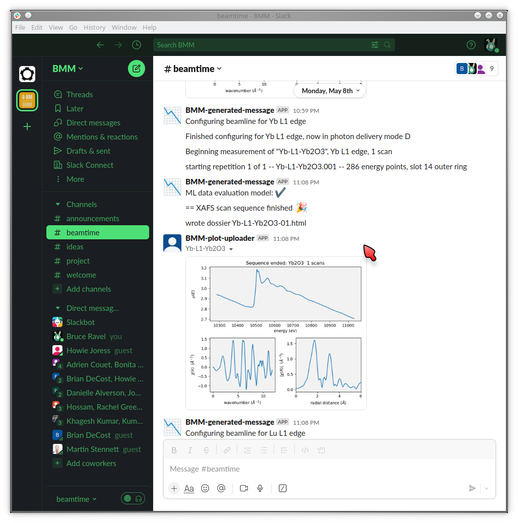
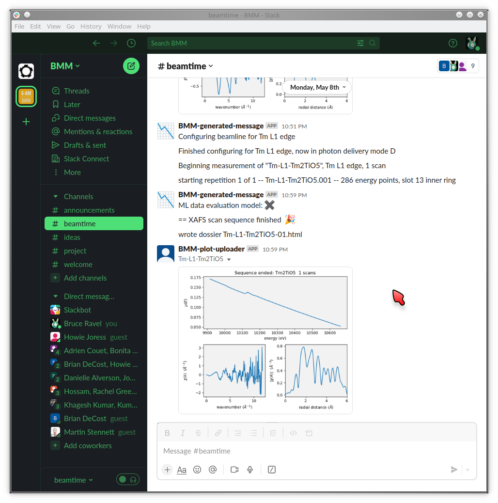
Fig. 9.1 Examples of data being evaluated as good (left) and bad (right) XAS data. The data on the left has an obvious edge step followed by oscillations. It, therefore, looks like XAFS data. The data on the right is an example of a marginal measurement. There is a step, but it’s not very big. Thus it looks like it might be a problematic measurement. It certainly is something that needs the attention of a human.#
This machine agent is a trained learning model. It uses a corpus of data measured at BMM and tagged by Bruce. The corpus includes hundreds of examples of good spectra and hundreds of examples of problematic measurements of all sorts. These are human-tagged as such and trained using a random forest classifier. Subsequent spectra are evaluated using this trained classifier. This evaluation happens upon completion of each XAFS scan repetition.
Experience so far with this model has been quite good. The training set is over 98% successful when tested against a subset of the training corpus. False positives (i.e. bad data identified as being good data) are exceedingly rare. False negatives (i.e. good data falsely identified as bad data) are much more common, happening most days.
That’s a fundamentally useful result. A false negative draws human attention to the beamline for a situation that might not require it. Frequent false positives would be much more problematic.
All negative results are logged so that the training model can be further refined by having a human tag each those negatives appropriately and adding them to the training corpus.
The random forest (RF) classifier was chosen because it is fairly simple and because it works well. Also tested were K-neighbors (KN) and a Multi-layer Perceptron (MLP). KN is certainly the simplest of the models tried – it is the model usually associated with the classic iris classification problem. It actually works quite well, although RF and MLP are both improvements. MLP was the suggestion of a local machine learning expert and performs similarly to RF on this trained data corpus.
9.10. Extract XRF spectra from fluorescence XAS#
BMM offers a handy tool for examining the XRF spectra of a fluorescence XAS scan on a point-by-point basis. Given the UID of a scan – which can be found in the dossier (Section 12.4) or in the header of the data file (Section 9.7) – you can plot the XRF spectrum at a given point in the scan.
xrfat(uid, energy)
Here, uid is a string containing the scan UID and energy is
one of the following:
an energy point in the scan range, the nearest energy point will be used
a negative integer, the energy point that many steps from the end of the scan will be used
a positive integer (smaller than the first energy value in the scan), the energy point that many steps from the beginning of the scan will be used
a list of any of the above, resulting in XRF spectra from each energy in the list being over-plotted.
For example,
xrfat(uid, -1)
will plot the XRF spectrum measured at the last point in the scan.
Here’s a good example of why this is useful. Some visitors to BMM were measuring a sample with a rather low concentration of neodymium (L3edge energy of 6208). The χ(k) data were noticeably distorted about 330 eV (or about 9.3 inverse Angstrom) above the edge. This corresponds to the K edge energy (about 6539) of Mn. We eventually determined that the BN used as a diluant was slightly contaminated with Mn.
Here are the plots from below and above the Mn K edge:
xrfat(uid, 6510)
xrfat(uid, 6560)
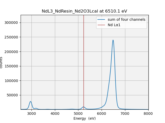
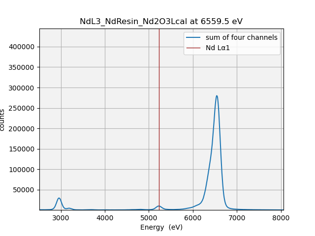
Fig. 9.2 (Left) The XRF spectra from the Nd-bearing sample measured at 6510 eV. (Right) The XRF spectra from the Nd-bearing sample measured at 6560 eV.#
Those don’t look very different. However, overplotting the two spectra and displaying on a log scale on the y-axis:
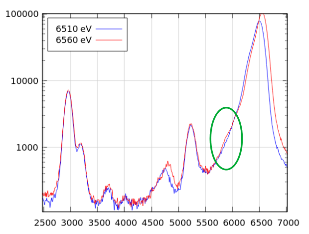
Fig. 9.3 The XRF spectra from the Nd-bearing sample measured at 6510 eV and at 6560 eV. There is a very small peak at the Mn Kα energy, marked by the green circle.#
While tiny, this Mn contamination had a noticeable impact on the
measured EXAFS data. This sort of forensic work is enabled by the
xrfat command.
The plots shown in Fig. 9.2 can be overplotted using the
list argument of energy, like so:
xrfat(uid, [6510, 6560])
The full signature of this function is
def xrfat(uid, energy=-1, xrffile=None, add=True, only=None, xmax=1500):
where
xrffileIf not None, is the name of the column data file to be written to the users
XRFfolder.addIf True, add the signals from the four channels
onlyIf specified as an integer (1, 2, 3, or 4), plot only that detector channel
xmaxSpecify the maximum energy plotted on the x-axis in units of energy above the measured fluorescence line energy
9.11. Reference spectra#
BMM has a wide variety of reference materials mounted in the reference position. The collection includes metal foils, metal powders, stable oxides, or other stable compound of 44 of the elements measurable at BMM.
The materials shown and listed below are always available for measurement. As part of the command for changing edge, the reference wheel will rotate to the position of the selected element. Every XAS scan will include the signal from the Ir chamber (whether any signal makes it to that detector depends on the sample being measured, of course).
The command for moving directly to a specific reference position is
RE(reference('Xx'))
where Xx is the one- or two-letter symbol of the element. See the
table below for the available elements.
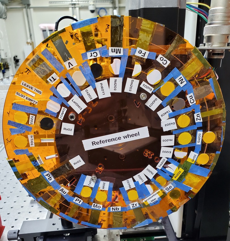
Fig. 9.4 The reference wheel at BMM#
Ring / slot |
Element |
Material |
Ring / slot |
Element |
Material |
|---|---|---|---|---|---|
Outer 1 |
empty |
for alignment |
Inner 1 |
Cs |
CsNO3 |
Outer 2 |
Ti |
foil |
Inner 2 |
La |
La(OH)3 |
Outer 3 |
V |
foil |
Inner 3 |
Ce |
Ce2O3 |
Outer 4 |
Cr |
foil |
Inner 4 |
Pr |
Pr6O11 |
Outer 5 |
Mn |
metal powder |
Inner 5 |
Nd |
Nd2O3 |
Outer 6 |
Fe |
foil |
Inner 6 |
Sm |
Sm2O3 |
Outer 7 |
Co |
foil |
Inner 7 |
Eu |
Eu2O3 |
Outer 8 |
Ni |
foil |
Inner 8 |
Gd |
Gd2O3 |
Outer 9 |
Cu |
foil |
Inner 9 |
Tb |
Tb4O9 |
Outer 10 |
Zn |
foil |
Inner 10 |
Dy |
Dy2O3 |
Outer 11 |
Ga |
Ga2O3 |
Inner 11 |
Ho |
Ho2O3 |
Outer 12 |
Ge |
GeO2 |
Inner 12 |
Er |
Er2O3 |
Outer 13 |
As |
As2O3 |
Inner 13 |
Tm |
Tm2O3 |
Outer 14 |
Se |
metal powder |
Inner 14 |
Yb |
Yb2O3 |
Outer 15 |
Br |
bromophenol blue |
Inner 15 |
Lu |
Lu2O3 |
Outer 16 |
Zr |
foil |
Inner 16 |
Rb |
RbCO3 |
Outer 17 |
Nb |
foil |
Inner 17 |
Ba |
<absent> |
Outer 18 |
Mo |
foil |
Inner 18 |
Hf |
HfO2 |
Outer 19 |
Pt |
foil |
Inner 19 |
Ta |
Ta2O5 |
Outer 20 |
Au |
foil |
Inner 20 |
W |
<absent> |
Outer 21 |
Pb |
foil |
Inner 21 |
Re |
ReO2 |
Outer 22 |
Bi |
BiO2 |
Inner 22 |
Os |
<absent> |
Outer 23 |
Sr |
SrTiO3 |
Inner 23 |
Sc |
metal powder |
Outer 24 |
Y |
foil |
Inner 24 |
Ru |
RuO2 |
For Th L3: Bi1 will be used (outer 22)
For U L3: Y K will be used (outer 24)
For Pu L3: Zr K will be used (outer 16)
Bromophenol blue: C19H10Br4O5S
Four elements are missing: Ba, W, & Os, and Ir.
See also BMM’s complete list of standard materials.
Here is a spreadsheet containing a sheet for for automated (see Section 11.3) measurements of the content of standards wheel.
