13. Managing the beamline

In this section, some recipes are provided for managing the beamline and meeting the needs and expectations of different experiments.

13.1. Starting and ending an experiment

When a new experiment begins, run the command:

BMMuser.begin_experiment(name='Betty Cooper', date='2019-02-29', gup=123456, saf=654321)

This will create that data folder and populate it with an experimental log (Section 12), write a template for a macro file (Section 9.6), configure the logger to write a user log file (Section 12.1) for this experiment, set the GUP and SAF numbers as metadata for output files, set up snapshot (Section 12.2) and dossier (Section 12.4) folders, and perform other experiment start-up chores.

The name should be the PI’s full name, preferably transliterated into normal ASCII. The date should be the starting day of the experiment in the YYYY-MM-DD format. The GUP and SAF numbers can be found on the posted safety approval form.

Once the experiment is finished, run this command:

BMMuser.end_experiment()

This will reset the logger and the BMMuser.folder variable and unset the GUP and SAF numbers.

13.2. Change energy

Changing energy is simple. Usually, it is as simple as doing

RE(change_edge('Fe'))

replacing the two-letter element symbol with the element you actually want to measure. This command will move the monochromator, put the photon delivery system in the correct mode, move the M2 bender to approximately the correct setting, run a rocking curve scan, optimize the slit height, move the reference foil holder to the correct position (if configured), and select the correct ROI channel (if configured).

If you want to reproduce this by hand, here is the command sequence:

1. First move the DCM to the new energy position. It is usually a good idea to move a bit above the target edge energy. Here’s an example for moving 50 eV above the iron K edge energy:

   RE(mv(dcm.energy, 7112+50))
   

2. Put the beamline in the correct photon delivery system mode. (See the table just above.) Continuing with the example of the iron K edge, for unfocused beam:

   RE(change_mode('E'))
   

   If the new edge energy is in the same energy range according to the table above, you can skip this step. For example, Mn and Fe are both in mode E (or mode C). The change_mode() command does not need to be run to move between those edges.

3. Measure a rocking curve scan (Sec 8.2) to verify that the second crystal of the rocking curve is parallel to the first crystal. This is more important for large energy changes. You may find that you can skip this step if you are changing between nearby edges.

   RE(rocking_curve())
   

   At the end of the scan, the mono pitch will be moved to the top of the rocking curve.

4. If using focused beam, make sure that the mirror bender is in the correct position. For focusing at the XAS table, m2_bender should be at about 212000 counts. For focusing at the position of the goniometer, m2_bender should be about 112000 counts.

   RE(mv(m2_bender, 212000))
   

5. Next, verify that the height of the hutch slits (Sec 8.2) is optimized for the beam height. In principle, this should be correct after changing photon delivery system mode. But it doesn’t hurt to verify.

   RE(slit_height())
   

   At the end of the scan, you will need to pluck the correct position from the plot.

6. Next, if you are using a reference foil, you should move the reference foil holder to the slot containing the correct foil. The command is something like:

   RE(reference('Fe'))
   

   choosing the correct element for your measurement.

7. Finally, select the correct ROI channel:

   BMMuser.verify_roi(xs, 'Fe', 'K')
   

As a reminder, here is the table of operating modes.

Table 13.1 Photon delivery modes

Mode	focused	energy range
A	✓	above 8 keV
B	✓	below 6 keV
C	✓	6 keV – 8 keV
D	✗	above 8 keV
E	✗	6 keV – 8 keV
F	✗	below 6 keV
XRD	✓	above 8 keV

13.3. Change crystals

Suppose you wanted to change from the Pt L3 edge (11564 eV) on the Si(111) crystal to the same energy on the Si(311) crystal.

RE(change_xtal('311'))

This will move the lateral motor of the DCM and optimize the roll and pitch of the second crystal. It will then move the DCM to the energy that you started at with the other crystal set and run a rocking curve scan.

Note that some of these motions can be a bit surprising in the sense that the monochromator will briefly report itself as being outside the normal operating range of the beamline. They will, however, eventually return to sensible places.

13.4. Change XAS → XRD

To move the photon delivery system to delivery of focused beam to the goniometer:

RE(change_edge('Ni', xrd=True, energy=8600))

The element symbol in the first argument is not actually used in any way when xrd=True is used, however the funtion requires something as its first argument. Setting xrd=True forces the focus=True and target=0 arguments to the change_edge() command to be set. This will move to the specified energy, place the photon delivery mode in XRD mode, optimize the second crystal and the slit height, and move to an approximately M2 bender position.

To do all of that by hand, you would do the follow commands:

RE(change_mode('XRD'))
RE(mv(dcm.energy, 8600))
RE(rocking_curve())
RE(slit_height())

This change of mode should have the beam in good focus at the position of the goniometer. 8600 eV is the nominal operating energy for the goniometer. If a higher energy is required, substitute the correct energy for 8600 in the second line.

Note

The I₀ chamber should be left in place. This will facilitate changing energy while doing scattering experiments. The flight path can be put in place at any time.

Todo

Determine look-up table for lower energy operations using both M2 and M3. This will require a new XAFS table and adjustments to the limit switches on m3_ydo and m3_ydi.

13.5. XAFS with Si(333)

Using the Si(111) monochromator, it is possible to use the third harmonic – the Si(333) reflection – to measure XAS with slightly higher energy resolution. In this section, we explain how to set up the beamline to measure the Ge K edge at 11103 eV using the Si(333).

You cannot use the change_edge() command to do this. Use of the Si(111) (or Si(311)) is hard-wired into that plan. You have to set up the beamline by hand.

First, put the photon delivery system in mode D (or mode A if using the focusing mirror):

RE(change_mode('D'))

Next, move the monochromator to a few 10s of eV above the absorption edge, as measured with the third harmonic. The Ge K edge is at 11103 eV, so we need to move the monochromator to 11103/3 = 3701 eV.

RE(mv(dcm.energy, (11103+27)/3))

or simply

RE(mv(dcm.energy, 3701+9))

This will put the third harmonic energy 27 eV above the Ge K edge.

Now, run a rocking curve scan:

RE(rocking_curve())

This will produce a plot that looks something like this:

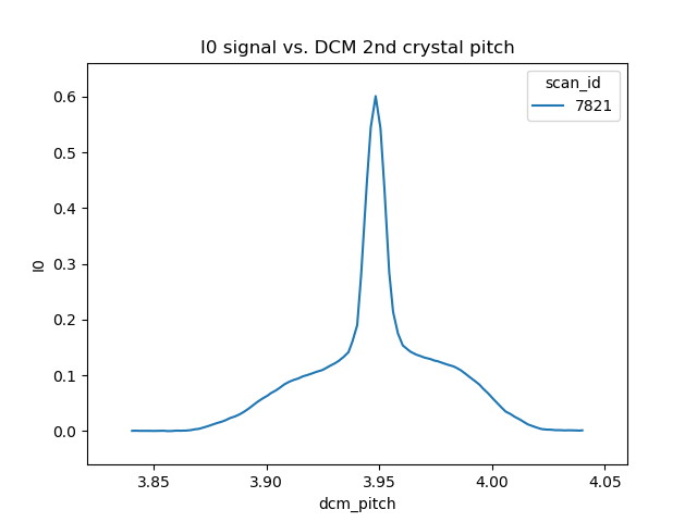
Fig. 13.1 A rocking curve scan with the photon delivery system in mode D and the mono at 3716 eV.

The broad base of this curve is the Si(111) rocking curve with photons at 3710 eV. The sharp spike in the middle is the Si(333) rocking curve with photons at 11130 eV.

Optimize the slit_height:

RE(slit_height())

You are ready to measure XAS with the Si(333) reflection!

Here’s an example scan.ini file for XANES of elemental Ge:

[scan]
experimenters = Bruce Ravel

filename      = Ge
sample        = elemental Ge, crystalline
prep          = standard sample
comment       = measured with Si(333) reflection, 25um Al foil in beam path before I0

ththth        = True
e0            = 11103
element       = Ge
edge          = K

nscans        = 1
start         = next

## mode is one of transmission, fluorescence, both, or reference
mode       = transmission

## Ge Si(333)
bounds     = -45    -18     -9      36    150
steps      =      9     0.9     0.3    0.9
times      =      0.5    0.5    0.5    0.5

Several things to note:

1. Note that the actual value for E0 is specified, not the divided-by-3 value.

2. Actual energy bounds and steps are specified, the xafs scan plan will convert them to appropriately sized steps for the Si(111).

3. By setting the 333 flag to True, the correct thing will happen, including writing the correct energy axis to the output data file.

4. The on-screen plot will show the fundamental – Si(111) – energy, however.

5. Also, you still need to set up the photon delivery system up by hand.

13.6. Motor controller kill switches

The MCS8 motor controllers supplied by FMBO have a kill switch for power cycling the Phytron amplifier cards. This is implemented by the vendor as connector plugged into the back of the chassis which shorts the two leads of the receptacle. To kill the amplifiers, this plug is removed and reinserted.

That’s fine, but the motor controllers are on top of the FOE – not a convenient location.

The new kill switch system uses DIODE to close the kill switch circuit. Two-conductor cable is run from each motor controller to a remote DIODE box mounted on the inboard wall of the end station.

The Bluesky interface is defined here

From the docstring of the class:

A simple interface to the DIODE kill switches for the Phytron
amplifiers on the FMBO Delta Tau motor controllers.

In the BMM DIODE box, these are implemented on channels 0 to 4 of
slot 4.

attributes
----------
dcm
  kill switch for MC02, monochromator
slits2
  kill switch for MC03, DM2 slits
m2
  kill switch for MC04, focusing mirror
m3
  kill switch for MC05, harmonic rejection mirror
dm3
  kill switch for MC06, hutch slits and diagnostics

methods
-------
kill(mc)
  disable Phytron
enable(mc)
  activate Phytron
cycle(mc)
  disable, wait 5 seconds, reactivate, then re-enable all motors

Specify the motor controller as a string, i.e. 'dcm', 'slits2', 'm2', 'm3', 'dm3'

Here is a common problem which is resolved using a kill switch.

   BMM E.111 [36] ▶ RE(mvr(m2.pitch, 0.05))
   INFO:BMM_logger:    Moving m2_pitch to 2.550

   Moving m2_pitch to 2.550
   ERROR:ophyd.objects:Motion failed: m2_yu is in an alarm state status=AlarmStatus.STATE severity=AlarmSeverity.MAJOR
   ERROR:ophyd.objects:Motion failed: m2_yu is in an alarm state status=AlarmStatus.STATE severity=AlarmSeverity.MAJOR
   ERROR:ophyd.objects:Motion failed: m2_ydi is in an alarm state status=AlarmStatus.STATE severity=AlarmSeverity.MAJOR
   ERROR:ophyd.objects:Motion failed: m2_ydi is in an alarm state status=AlarmStatus.STATE severity=AlarmSeverity.MAJOR
   Out[36]: ()

This is telling you that the amplifiers for two of the M2 jacks
went into an alarm state. In the vast majority of cases, this
simply requires killing and reactivating those amplifiers.

The solution to this one is:

   BMM E.111 [1] ▶ ks.cycle('m2')
   Cycling amplifiers on m2 motor controller
   killing amplifiers
   reactivating amplifiers
   enabling motors

13.6.1. Old kill switch system

There is a row of switches on rack D, the rack next to the control station, that are used to disable the amplifiers for the MCS8 motor controllers. The cabling for this system still exists, but is not plugged into the controllers. Should the DIODE system somehow fail, this can be redeployed easily.

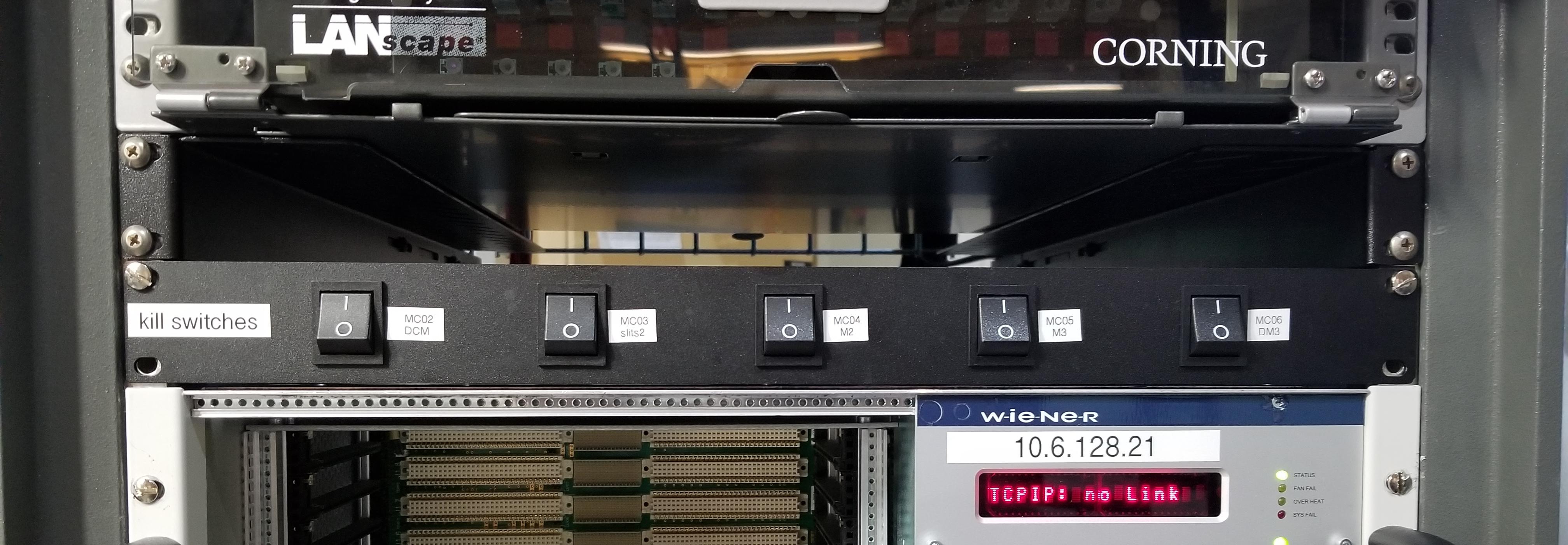
Fig. 13.2 The manual kill switch system

When you suspect that a motor has an amplifier fault, toggle the appropriate switch to the off position. Wait 10 seconds (to be very safe…). Then toggle the switch back to the on position. The motor should be ready to go. These switches replace the shorted plugs that came attached to the “disable” port on the back side of the MCS8s.

MCS8	RGA label	RGD label	motors
MC02	6BM-100149-RG:A1-PT1B3-A	6BM-100149-RG:A1-PT1B3-B	DCM
MC03	6BM-100150-RG:A1-PT1B3-A	6BM-100150-RG:A1-PT1B3-B	slits2
MC04	6BM-100151-RG:A1-PT1B3-A	6BM-100151-RG:A1-PT1B3-B	M2 + DM2 FS
MC05	6BM-100152-RG:A1-PT1B3-A	6BM-100152-RG:A1-PT1B3-B	M3 + Filters
MC06		<installed, not yet labeled>	DM3 (bct,bpm,fs,foils)+ Slits3

In the situation where toggling the switch does not clear the amplifier fault, the next troubleshooting step is to power cycle the MCS8. This is done by toggling the red, illuminated switch on the front of the MCS8. Wait for the red amplifier lights to stop flickering after turning off the MCS8, then turn the MCS8 back on.

After power cycling the MCS8, it is necessary to re-home all the motors controlled by the MCS8.

13.6.2. MCS8 Connector

The disable plug on the back of the MCS8 controllers is a Binder RS connector, part number 468-885. Here’s an example.

And here is the wiring diagram. Short the prongs on the side opposite to the alignment groove.

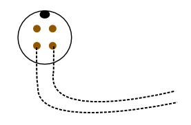
Tutorial for how to put together the Binder connectors: PDF

13.7. Windows VM and BioLogic

We use the BioLogic EC_lab software to run the VSP-300 potentiostat. Since there is not a dedicated Windows machine at BMM, EC-Lab is run on a virtual machine that is spun up when needed.

Similarly, Hiden’s control software is a Window’s only produce. It is run on the same firtual machine.

Here are the instructions for starting and interacting with the the VM.

13.7.1. Starting the virtual machine

• At a command line, do rdesktop xf06bm-srv2 &

• This will open a new window and display a Windows login screen. Normal BNL credentials do not work. Log in as user xf06bm using the password known by beamline staff.

• The Windows desktop might start with a full-screen management application that looks like the figure below. You can close or minimize that window.

• Double-click on the EC-lab or Hiden icon.

• Do some electrochemistry or mass spectrometry.

• Save your electrochemistry or mass spectrometry data to the assets folder as explained below.

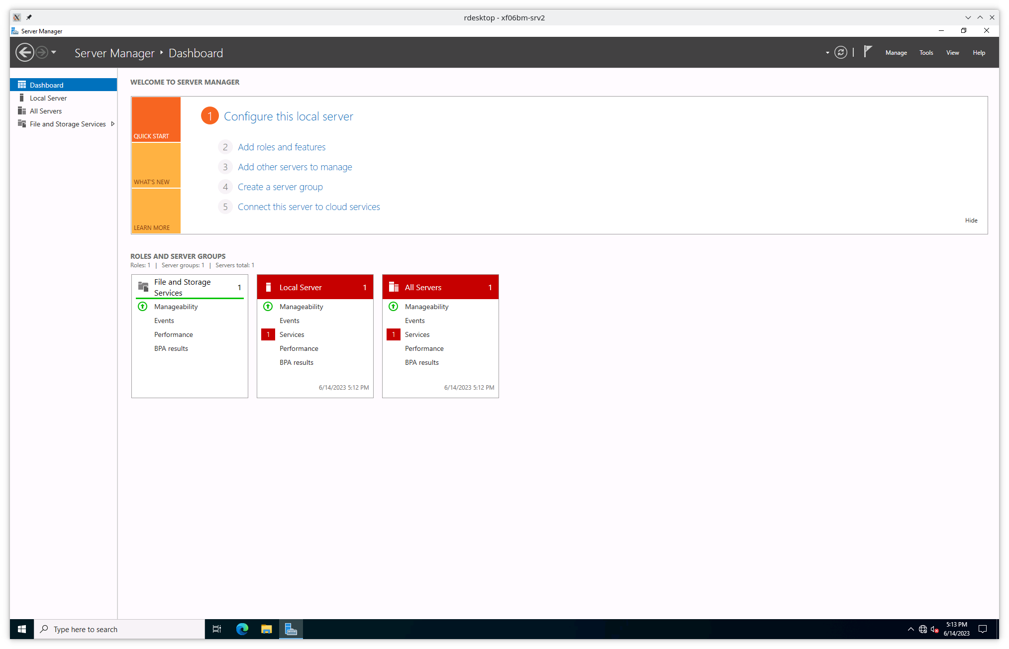
Fig. 13.3 VM management window. You can minimize or close this.

13.7.2. Storing electrochemistry or mass spectrometry data

The Windows VM has permission to connect to central storage with permissions to write files from EC-lab or the Hiden software to the correct location.

To start a new experiment, you first have to disconnect the old drive (if connected). This is likely mounted as the Z: drive.

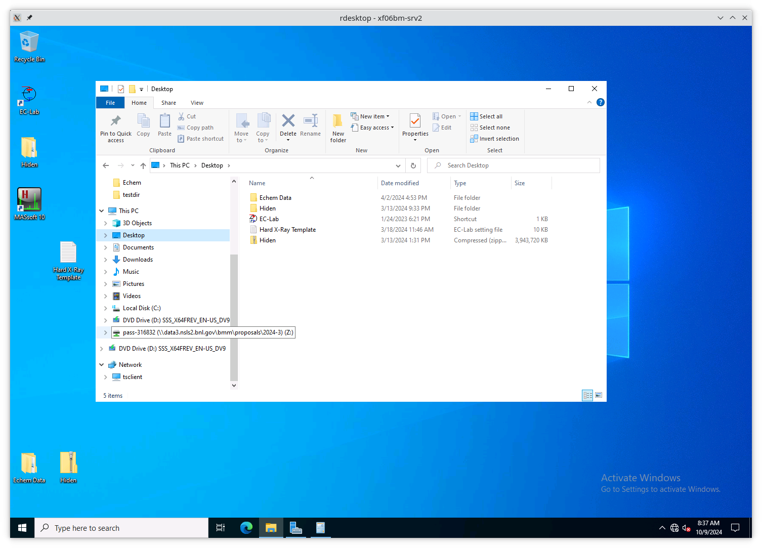
Fig. 13.4 An example of a stale folder from a previous experiment mounted as the Z: drive.

Disconnect the stale Z: drive by right clicking on its entry in the side bar and selecting “Disconnect”.

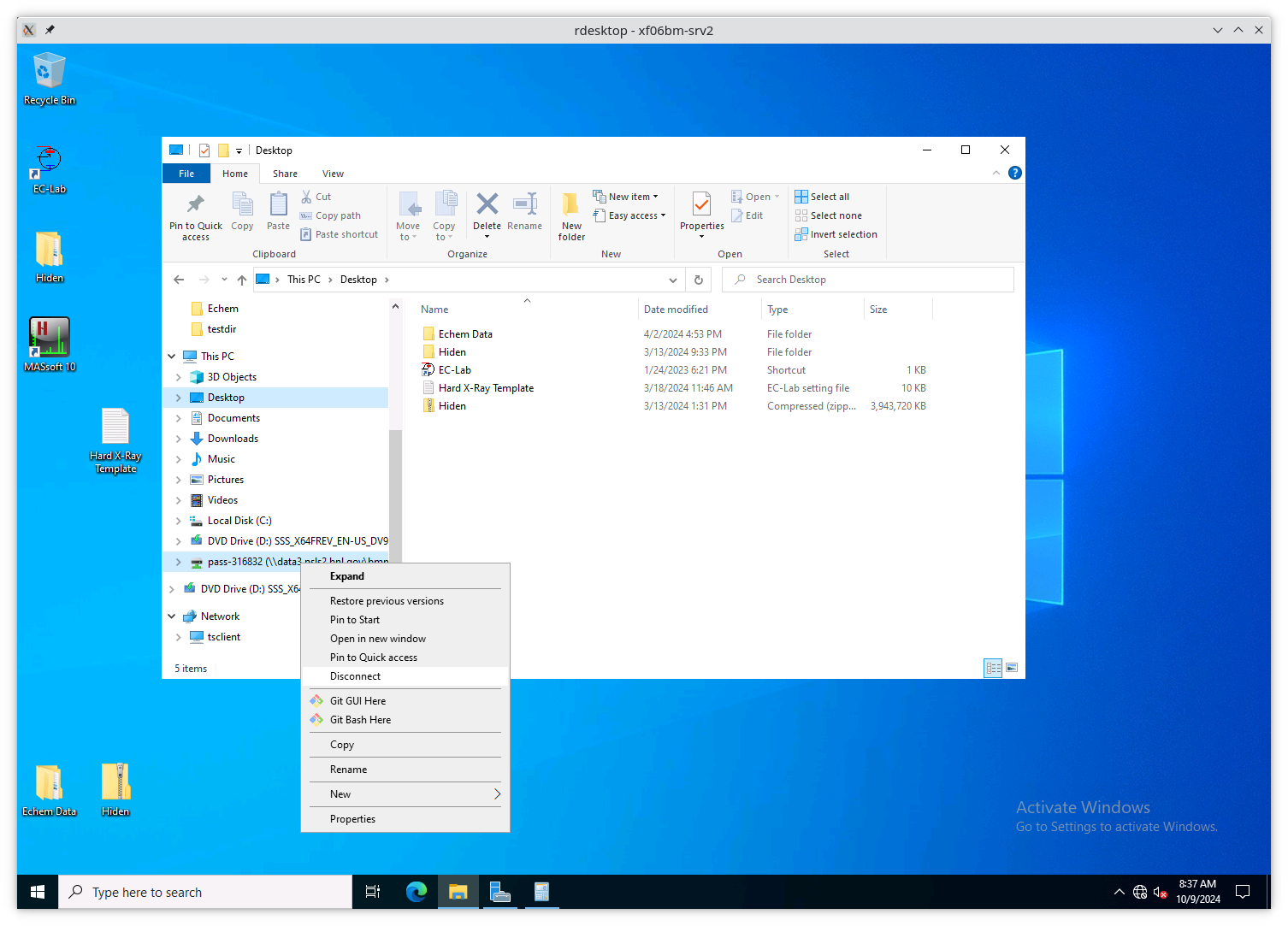
Fig. 13.5 Disconnect the stale Z: drive.

Next, click on “This PC” in the sidebar, then click on the button that says “Map network drive”.

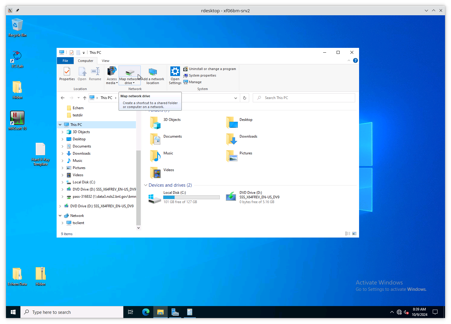
Fig. 13.6 Map a new network drive to the VM.

On the “Map Network Drive” page, you need to fill in the path to the current experiment’s proposal folder. Suppose the current cycle is 2024-3 and the current proposal number is 316832. Using Z: as the drive letter, enter the following as the “Folder”

\\data3.nsls2.bnl.gov\bmm\proposals\2024-3\pass-316832

Note that the backslashes are important. Also substitute the correct cycle and proposal numbers.

Be sure to leave “Reconnect at sign-in” checked. Note that “Connect using different credentials” should be unchecked.

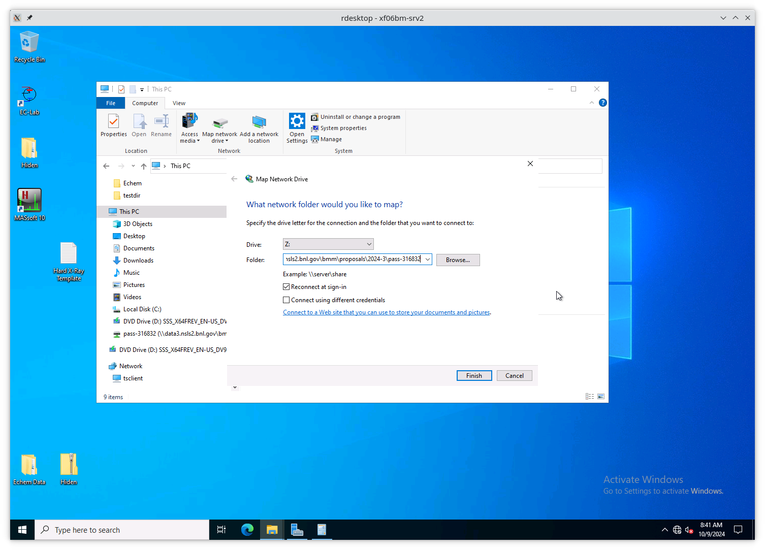
Fig. 13.7 Map a new network drive to the VM.

Click the finish button. The connection will take several seconds, but then the new entry will show up in the side bar.

The new network drive can now be clicked into.

Configure EC-lab to write its data files into the assets\vsp300-1 folder.

Configure the Hiden software to write its data files into the assets\hpr20-1 folder.

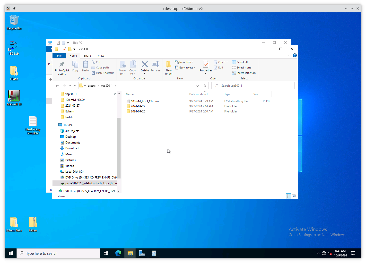
Fig. 13.8 The assets\vsp300-1 folder is the correct place for data from EC-lab to be written. The assets\hpr20-1 folder is the correct place for data from the Hiden to be written.

By following this procedure, the electrochemistry data from EC-lab and mass spectrometry data from the Hiden will be available to the user in the same manner as their XAS data (Section 4).

13.8. Calibrate the mono

The typical calibration procedure involves measuring the angular position of the Bragg axis for the edge energies of 10 metals: Fe, Co, Ni, Cu, Zn, Pt, Au, Pb, Nb, and Mo.

The tabulated values of edge energies from Table 1 in Kraft, et al. are used in the calibration.

1. Be sure that all 10 of these elements are actually mounted on the reference wheel and configured in the xafs_ref.mapping dict. (They should be. It would be very unusual for any of these foils to have been removed from the reference wheel.)

2. Run the command

   RE(calibrate(mono='111'))
   

   Use the mono='311' argument for the Si(311) monochromator. This will, in sequence, move to each edge and measure a XANES scan over a wide enough range that it should cover the edge (unless the mono is currently calibrated VERY wrongly). This will write a file called edges111.ini (or edges3111.ini). Each XANES scan uses the file /home/xf06bm/Data/Staff/mono_calibration/cal.ini as the INI file. Edge appropriate command line parameters will be added by the calibrate() plan.

3. Examine the data in athena. Make sure E₀ is selected correctly for all 10 edges. Copy those values into the first column of edges111.ini (or edges311.ini).

   Attention

   It is no longer necessary to compute the angular positions of the monochromator. Those will be computed from the edge energy values you edited into the INI file by hand.

   Todo

   Implement on-the-fly determination of E₀ to obviate the step of editing the INI file. Pb is tricky. Nb and Mo are kind of tricky.

4. Run the command

   calibrate_mono(mono='111')
   

   (or use the '311' argument). This will show the fitting results and plot the best fit. It will also print in a text box instructions for modifying the BMM/dcm-parameters.py file to use the new calibration values.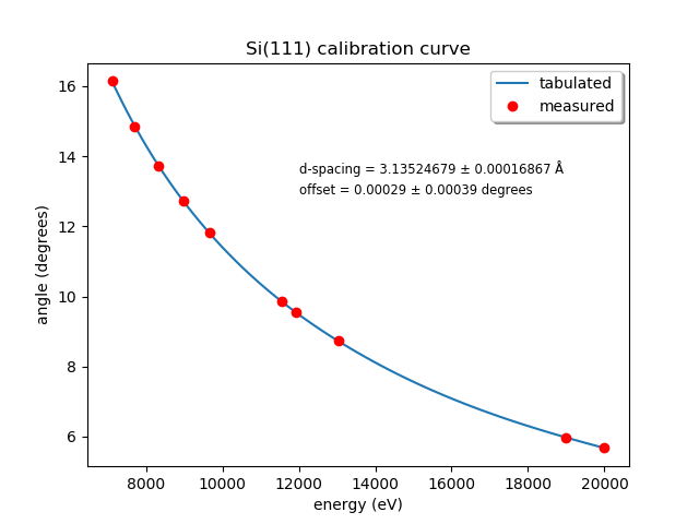

   

   Fig. 13.9 Example calibration curve

5. Edit BMM/dcm-parameters.py as indicated.

6. Do

   %run -i 'home/xf06bm/.ipython/profile_collection/startup/BMM/dcm-parameters.py'
   

   then do

   dcm.set_crystal()
   

   Or simply restart bsui, which is usually the easier thing.

7. Finally, do

   calibrate_pitch(mono='111')
   

   This performs a simple linear fit to the rocking curve peak positions for dcm_pitch found at each edge. Use the fitted slope and offset to modify approximate_pitch in BMM/functions.py.

The mono should now be correctly calibrated using the new calibration parameters.

13.9. Provision a new beamline computer

This is a list of notes on how to finish the provisioning of a new beamline computer.

Firstly, make sure that /nsls2/data is a symlink to /nsls2/data3. If it is not, ask for help from DSSI.

13.9.1. install additional packages

• plasma-desktop (just … better)

• redis (essential for operation of bsui)

• most (used as the pager in BMM’s bsui profile)

• ag (powerful ack-like grep alternative)

• fswebcam (used to capture analog pinhole camera)

• demeter and perl-Graphics-GnuplotIF (something silly, no doubt)

• slack (communications)

• ark (compression, useful in file manager)

To install these, do:

dzdo dnf install redis most ag fswebcam demeter perl-Graphics-GnuplotIF slack ark
dzdo dnf install --skip-broken --nobest @kde-desktop

The second command installs the KDE metapackage, skipping missing packages.

To finish installing sddm, do

dzdo systemctl stop gdm
dzdo systemctl start sddm

13.9.2. Desktop wallpaper

This may not be provisioned correctly out of the box. Find the beamline wallpapers in /usr/share/nsls2/wallpapers/beamlines.

Right click on the desktop and select “Configure Desktop and Wallpaper”. Click on “Add Image” and navigate to the folder above.

13.9.3. Things to install from git

• BMM stuff: git clone git@github.com:NSLS-II-BMM/BMM-beamline-configuration.git + then, cd ~/bin and ln -s ~/git/BMM-beamline-configuration/tools/run-cadashboard

• BMM user manual: git clone git@github.com:NSLS-II-BMM/BeamlineManual.git

• BMM standards: git clone git@github.com:NSLS-II-BMM/bmm-standards.git

• Switch visualization: git clone git@github.com:NSLS-II-BMM/switch-pretty-printer.git

Also do cd ~/bin and ln -s ~/.ipython/profile_collection/startup/consumer/run-consumer

13.9.4. Workspace folders

Make the local data collection folders. The BMMuser.begin_experiment() command (Section 13.1) will make symlinks under those folders to the correct place on central storage.

mkdir ~/Workspace
mkdir ~/Workspace/Visitors
mkdir ~/Workspace/Staff

13.10. Manage Silicon Drift Detectors

The assumption in the data acquisition system is that one of the three silicon drift detectors will be the primary detector in an experiment. At the bsui command line (or in queueserver) the xs symbol should point at the correct detector. Also, a parameter is set in Redis allowing other processes (such as the Kafka plotting agent) to know which detector to be paying attention to.

xs = xspress3_set_detector(7)

where the argument to xspress3_set_detector is 1, 4, or 7. Since October 2024, use of the seven element detector is the default.

This sets xs to the selected detector object – xs1, xs4, or xs7.

Also set is the Redis parameter BMM:xspress3, which is set to 1, 4, or 7 (and represented as a b-string).

n_elements = int(rkvs.get('BMM:xspress3'))