
6. Moving and querying motors#
To get an overview of the state of the beamline motors, do %m at
the bsui command line. Here is an example:
In [1897]: %m
==============================================================================
Energy = 19300.1   reflection = Si(111)   mode = fixed
     Bragg =  5.87946   2nd Xtal Perp = 15.0792   2nd Xtal Para = 146.4328

M2
     vertical =   6.000 mm           YU  =   6.000
     lateral  =   0.000 mm           YDO =   6.000
     pitch    =   0.000 mrad         YDI =   6.000
     roll     =  -0.001 mrad         XU  =  -0.129
     yaw      =   0.200 mrad         XD  =   0.129

M3
     vertical =   0.000 mm           YU  =  -1.167
     lateral  =  15.001 mm           YDO =   1.167
     pitch    =   3.500 mrad         YDI =   1.167
     roll     =   0.000 mrad         XU  =  15.001
     yaw      =   0.001 mrad         XD  =  15.001

Slits3:   vsize  vcenter  hsize   hcenter     top    bottom    outboard  inboard
          1.350   0.000   8.000  -0.000      0.675   -0.675    4.000   -4.000

DM3_BCT:  45.004 mm

XAFS table:
     vertical  pitch    roll   YU     YDO     YDI
     132.000   0.000   0.000 132.000 132.000 132.000

XAFS stages:
          x        y     roll    pitch    linxs    roth    wheel     rots
        9.224  115.000   0.840   0.000  -45.000    0.000  -59.000    0.000
==============================================================================
6.1. Sample stages#
These stages sit on top of the XAFS optical table.
motor |
type |
units |
notes |
directions |
|---|---|---|---|---|
|
linear |
mm |
main sample stage |
+ outboard, - inboard |
|
linear |
mm |
main sample stage |
+ up, - down |
|
linear |
mm |
detector mount |
+ away from sample, - closer |
|
linear |
mm |
detector mount |
+ uo, - down |
|
linear |
mm |
detector mount |
+ downstream, - upstream |
|
rotary |
degrees |
ex situ sample wheel |
+ clockwise, - widdershins |
|
linear |
mm |
ref wheel vertical |
+ up, - down |
|
rotary |
degrees |
reference stage |
+ clockwise, - widdershins |
|
linear |
mm |
reference stage |
+ outboard, - inboard |
|
linear |
mm |
reference stage |
+ up, - down |
|
tilt |
degrees |
Huber tilt stage |
+ more positive |
|
tilt |
degrees |
Huber tilt stage |
+ more positive |
|
rotary |
degrees |
small rotary stage |
+ clockwise, - widdershins |
|
rotary |
degrees |
g.a. rotary stage |
+ clockwise, - widdershins |
|
linear |
mm |
u.s table jack |
+ up, - down |
|
linear |
mm |
d.s o.b. table jack |
+ up, - down |
|
linear |
mm |
d.s i.b. table jack |
+ up, - down |
|
linear |
mm |
spare linear stage |
g.a. = glancing angle ● o.b. = outboard ● i.b. = inboard ● u.s. = upstream ● d.s. = downstream
Here are some photos identifying these axes:
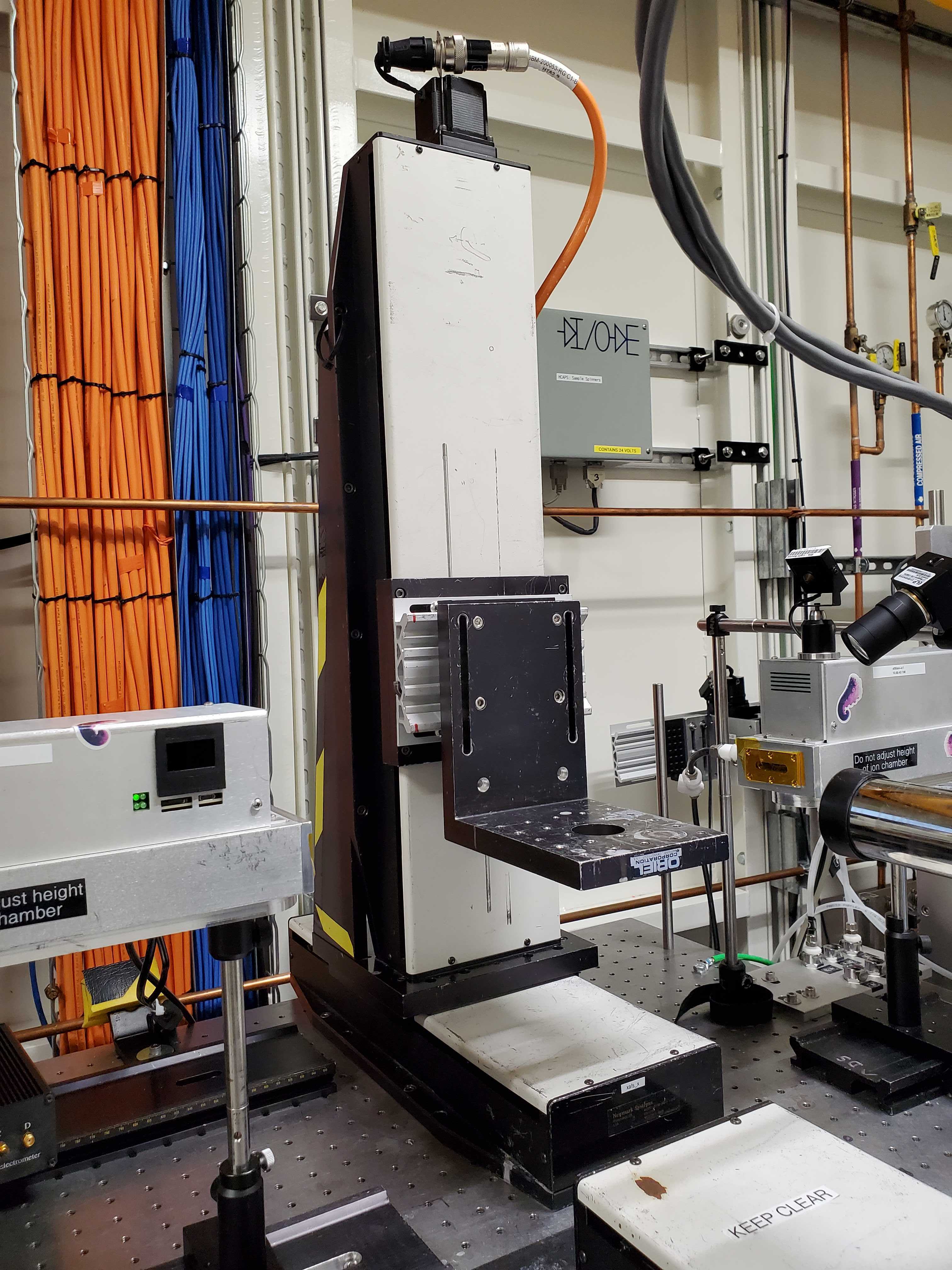
Fig. 6.1 The two-axis main sample stage: xafs_x and xafs_y.#
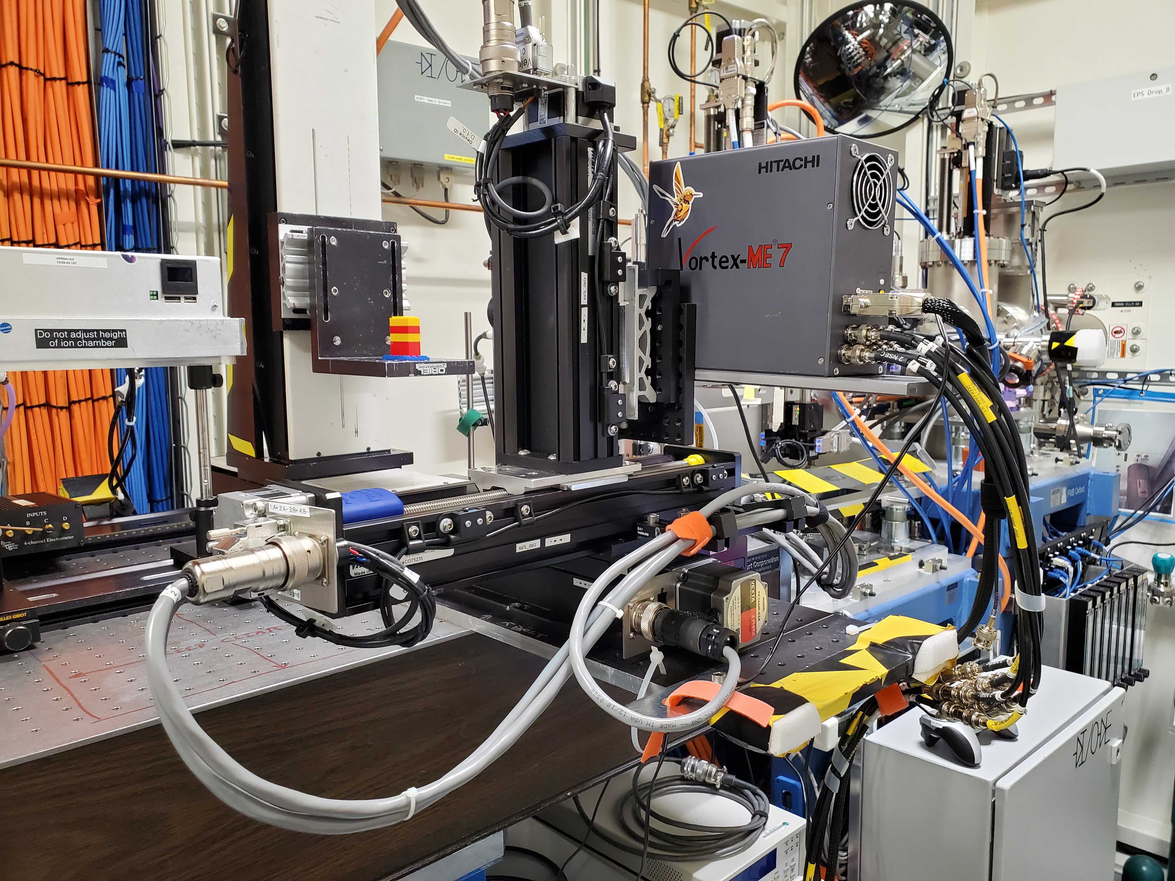
Fig. 6.2 The three-axis stage holding the fluorescence detector:
xafs_detx, xafs_dety, and xafs_detz.#

Fig. 6.3 The three-axis stage holding the reference wheel: xafs_ref,
xafs_refx, and xafs_refy.#
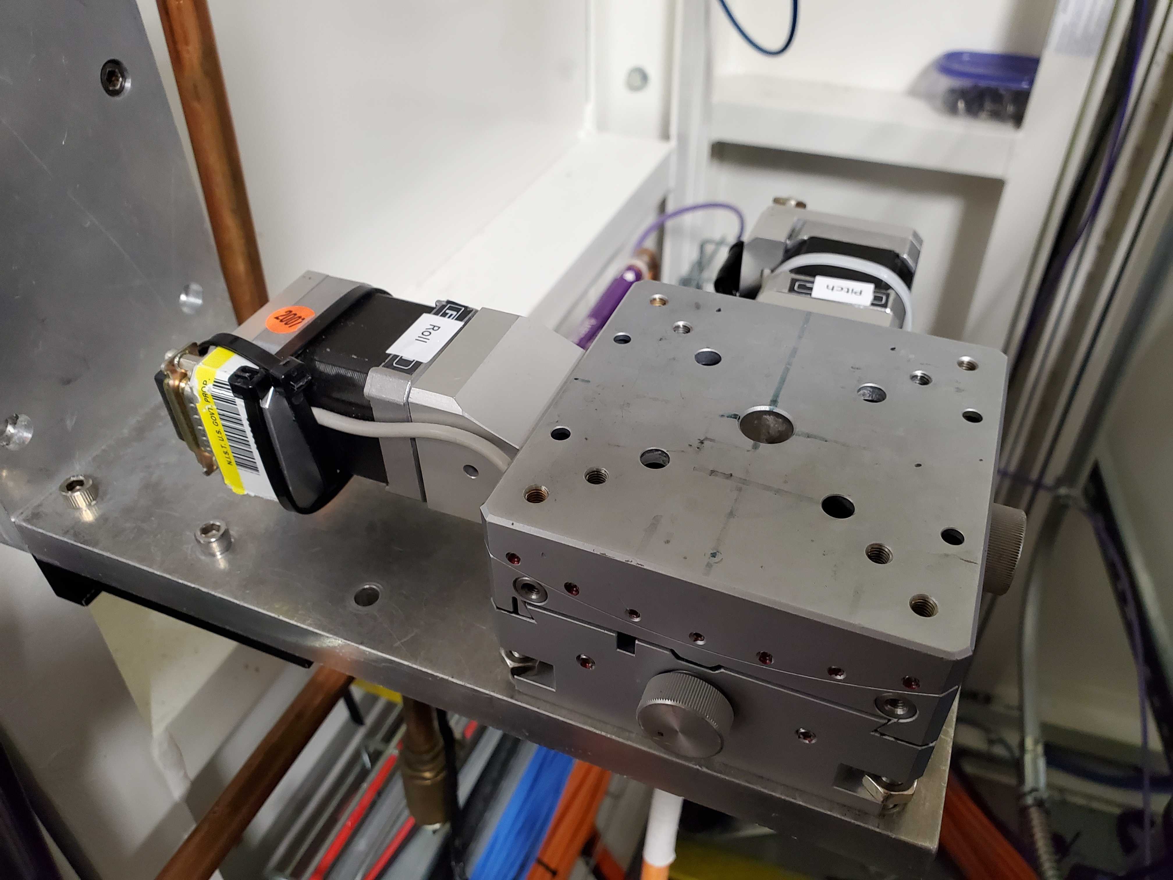
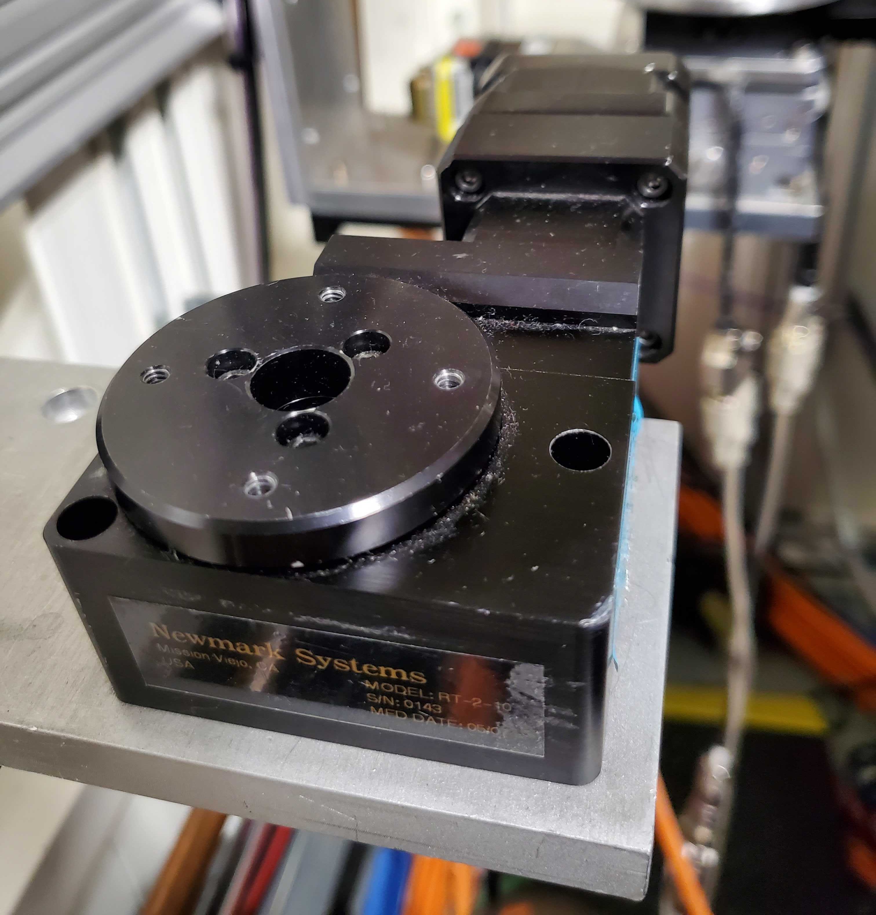
Fig. 6.4 (Left) The pitch and roll stage: xafs_pitch and xafs_roll.
(Right) The small rotation stage: xafs_rots#

Fig. 6.5 The glancing angle rotary stage, here sitting on top of the pitch
and roll stage: xafs_garot.#
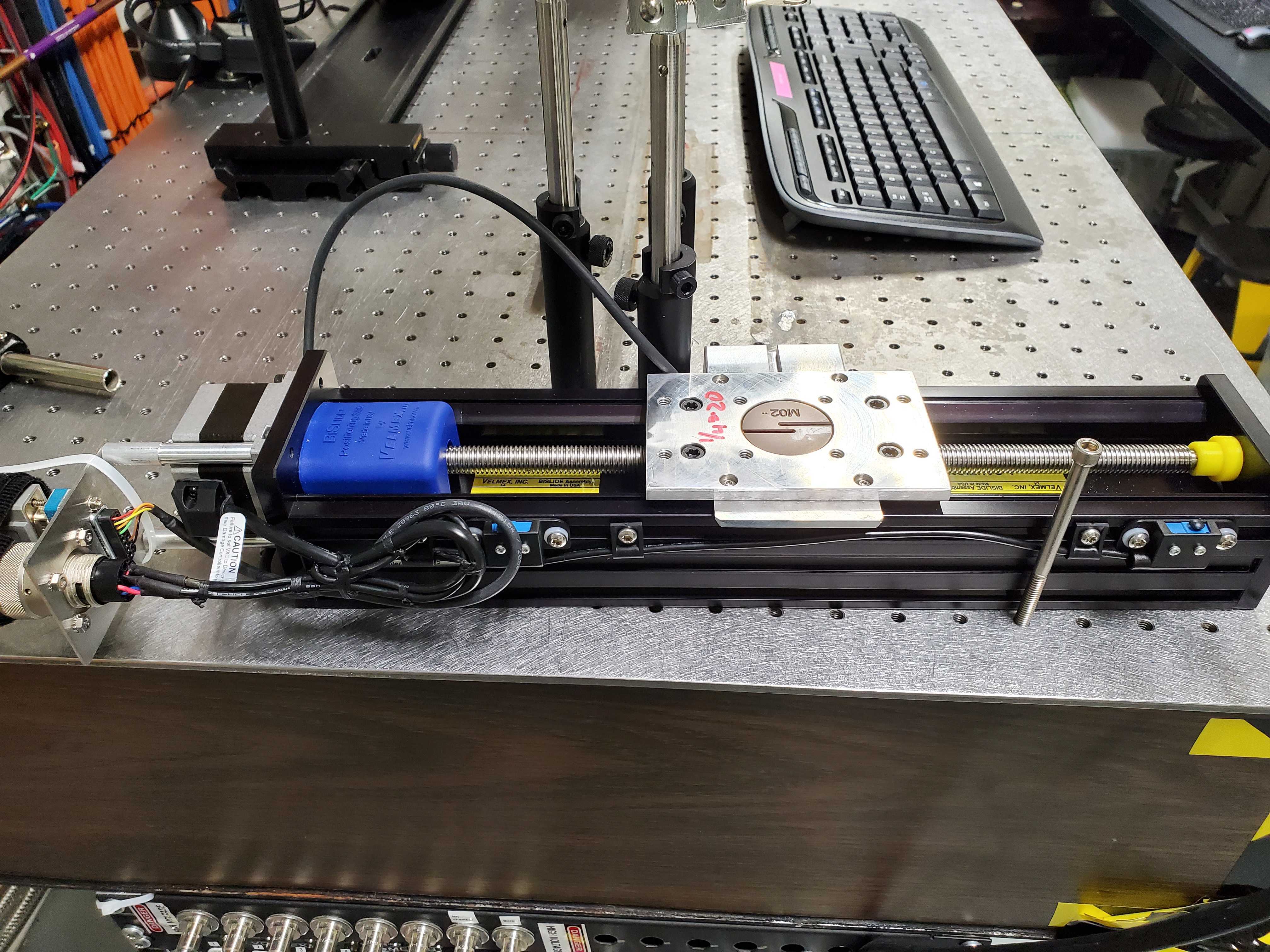
Fig. 6.6 The spare linear stage: xafs_spare.#
6.2. Basic motor commands#
Configuration and position of the motors can be queried easily. In
the following examples, the xafs_y motor is used. The commands
are the same for all sample stage motors.
- Querying position
The position of a motor can be queried with a command line like
%w xafs_y
or
xafs_y.position
- Moving to a new position
Always move motors through the run engine, for example:
RE(mvr(xafs_y, 10))
mvris the relative move command – the numerical argument is the amount by which the motor will move from the current position.mv, as in:RE(mv(xafs_y, 37.63))
is the absolute move command. The numerical argument is the position to which the motor will move.
- Moving to a new position in a plan
To move a sample stage as part of a macro (Section 9.6) , do:
yield from mv(xafs_y, 37.36)
You can combine motions of two or more motors in a single synchronous movement:
yield from mv(xafs_y, 37.36, xafs_x, 15.79)
Similarly:
yield from mvr(xafs_y, 5)
- Querying soft limits
To know the soft limits on a sample stage, do
xafs_y.limitsorxafs_y.llm.get()orxafs_y.hlm.get()to query the low or high limits individually.- Setting soft limits
To set the soft limits on a sample stage, do something like
xafs_y.llm.put(5)orxafs_y.hlm.put(85)- Reference wheel
The reference stage (Section 7.2.1) is a rotation stage with a sample wheel holding up to 48 reference foils. It is calibrated such that the beam passes through the center of a slot every 15 degrees. The slots are indexed such that they can be accessed by the symbol of the element being measured. To move to a new reference foil:
RE(reference('Fe'))
To see the available foils, do
%seor look at the value ofxafs_ref.mapping.See Section 9.11 for a full explanation of the the reference wheel contents.
Here is a complete list of standards in BMM’s collection. These standards are mounted on sample wheels and stored in the hutch for ready access by users.
6.3. Sample wheel#
The xafs_wheel motor is a rotary stage that is typically mounted
on the XY stage. It can be mounted face-on to the beam or at 45
degrees for use with the fluorescence detector.
Sample plates laser cut from plastic sheet (initially we used Delrin, since COVID made supply difficult, we use whatever we can get) are attached to the rotation stage. The single-ring version of these plates have 24 slots arranged around the periphery, evenly spaced 15 degree apart. The double-ring version has concentric rings of 24 slots each. These are still 15 degrees apart. The radius of the outer ring is 26 mm larger than the radius of the inner ring.
While you can move from slot to slot in increments of 15 degrees, i.e.
RE(mvr(xafs_wheel, 15*3))
it is somewhat easier to move by slot number. The sample plates are cut with sample numbers for slots 1, 7, 13, and 19, making it clear which slot is which. The wheel is mounted such that the numbers can be read normally on the side facing the beam.
To move, for instance, to slot 5, do:
RE(slot(5))
In a macro, do
yield from slot(5)
To move to the inner or outer ring, do
RE(xafs_wheel.inner())
RE(xafs_wheel.outer())
This translates xafs_x by ±26 mm.
In a macro, do
yield from xafs_wheel.inner()
yield from xafs_wheel.outer()
6.4. Glancing angle stage#
The glancing angle stage, shown in Figure 6.7, can hold up to eight samples and allows each sample to spin independently. The spinning allows spurious diffraction from a crystalline substrate into the fluorescence detector to be suppressed.
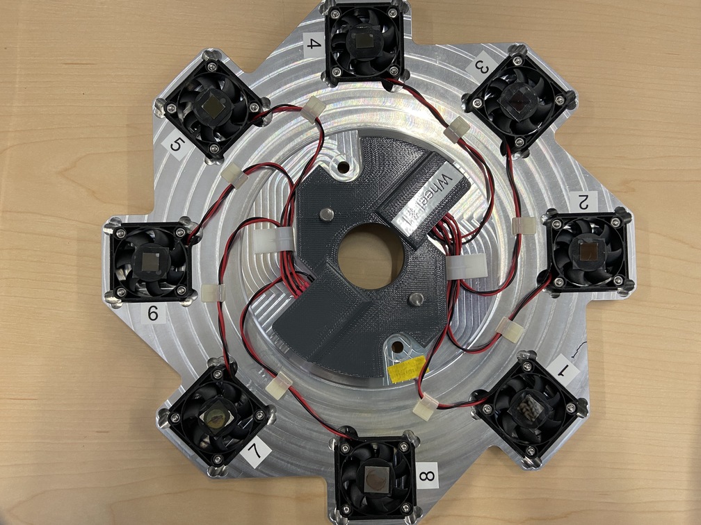
Fig. 6.7 The glancing angle stage with 8 sample positions.#
To move to a sample position:
RE(ga.to(3))
where the argument is a number from 1 to 8, as shown by the labels in Figure 6.7. This command will turn off all other spinners, rotate that sample into the beam path, and start the sample spinning.
To turn a spinner on or off, where the argument is a number from 1 to 8:
RE(ga.on(3))
RE(ga.off(3))
To turn off all spinners:
RE(ga.alloff())
In a plan:
yield from ga.on_plan()
yield from ga.off_plan()
yield from ga.alloff_plan()
6.4.1. Sample alignment#
A sample is aligned into the beam by moving the tilt stage to an approximately flat position:
RE(mv(xafs_pitch(0))
Then performing the following sequence:
RE(linescan(xafs_y, 'It', -1, 1, 41))
RE(linescan(xafs_pitch, 'It', -2, 2, 41))
At the and of the xafs_y scan, pick the position halfway down the
edge in the It signal. At the end of the xafs_pitch scan, select
the peak position. This will place the sample such that it is flat
relative to the incident beam direction and halfway blocking the beam.
You may choose to iterate those two scans.
Next move the sample to the measurement angle. Suppose the measurement angle is 2.5 degrees:
RE(mv(xafs_pitch, 2.5))
Finally, position the sample so that the beam is hitting the center of the sample:
RE(linescan(xafs_y, 'If', -1, 1, 41))
Since the sample is not at the eucentric of the tilt stage, this final
vertical scan is always necessary. When first aligning the sample,
you may need to center the sample in xafs_x as well:
RE(linescan(xafs_x, 'If', -6, 6, 41))
You will almost certainly need to scan over a longer range. Make sure the detector is retracted far enough to allow for this motion.
6.4.2. Automated alignment#
The sequence described above can be automated in many cases:
RE(ga.auto_align(2.5))
This will run the sequence of alignment scans described above,
pitching the sample to the user-specified angle before the vertical
scan measuring the fluorescence signal. This works by fitting an
error function to the xafs_y scan versus It, selecting the peak of
the pitch scan, then selecting the peak of the xafs_y scan versus
fluorescence.
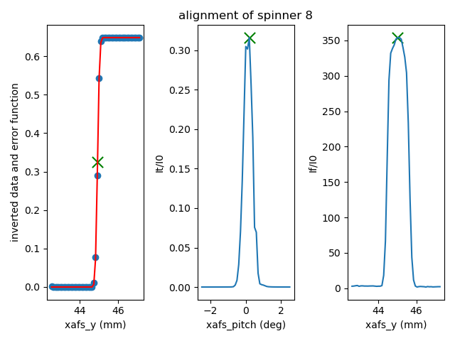
Fig. 6.8 If all goes well, the result of the sample alignment looks like this. A picture like this is posted to Slack (Section 1.3.2).#
For very flat samples which are square or circular and about 5mm across or larger, this alignment algorithm is very robust. For oddly shaped samples, verify that the automation works before relying upon it. Otherwise, simply do the alignment by hand.
6.5. Table motors#
Typically, table motors are not moved individually. When changing
photon delivery system modes (Section 7.8.1), the
table should be put into the correct orientation such that the beam
passes through the center of the ion chambers. It is very easy to put
the beamline in a confusing state by changing the table motors outside
of the change_mode() command.
The lateral table motors – and its yaw – are normally disabled.
motor |
units |
notes |
|---|---|---|
xafs_yu |
mm |
upstream table jack |
xafs_ydi |
mm |
downstream, inboard table jack |
xafs_ydo |
mm |
downstream, outboard table jack |
xafs_vertical |
mm |
coordinated linear motion |
xafs_pitch |
degrees |
coordinated table pitch |
xafs_roll |
degrees |
coordinated table roll |
- Querying table position
The position of any motor can be queried with a command line like
%w xafs_table.- Coordinated table movement
RE(table_height(mode='A')): Move the table to its position for a specified mode, the modes (see Section 7.8.1) are'A','B','C','D','E', and'F'.RE(table_height(by=amount)): Move the table vertically by an amount. This moves the three vertical motors the same amount.RE(table_height(pitch=adjustment)): Move the front by the specified amount, move the back the same in the opposite direction. I.e. adjust the pitch of the table, except that the adjustment is in mm units, not degrees.
- Moving table motors
The normal movement commands work on the real and virtual motors, e.g.:
RE(mvr(xafs_ydi, 3))
RE(mv(xafs_vertical, 107))
Again, this is rarely necessary. The mode changing plan should leave the table in the correct location for your experiment.
All table movements are recorded in the experimental log (Section 12).
6.6. Examine Motor Axes#
Some BlueSky functionality related to the axes controlled by the FMBO MCS8 motor controllers. These include:
Collimating mirror (
m1_*)Filter assemblies (
dm1_*)Monochromator (
dcm_*)Second diagnostic module (
dm2_*)Focusing mirror (
m2_*)Harmonic rejection mirror (
m3_*)Third diagnostic module (
dm3_*)
(38 axes motors in total) but not any of the end station motors
(xafs_*), which are run using NSLS-II standard GeoBricks.
- Homing
Any of these axes can be homed with, for example,
dm3_bct.home()- Summarize the status of a motor
To show the values of all the status flags, for example,
dm3_bct.status()- Which motors have been homed?
Do this command:
homed()- Which motors have their amplifiers enabled?
Do this command:
ampen()